Time: The Fourth Dimension in Multiomics Data Analysis

Incorporating time-dependent relationships in multiomics data analysis

Enjoyed this piece? Show your support by tapping the ❤️ in the header above. It’s a small gesture that goes a long way in helping me understand what you value and in growing this newsletter. Thanks so much!

---

Last month, a colleague showed me RNA-seq data from muscle biopsies taken shortly after exercise alongside proteomic measurements from the same tissue samples. The transcriptomic data screamed adaptation. Genes for mitochondrial biogenesis, protein synthesis, and multiple members of the NR4A family were all up-regualted compared to baseline conditions. But, the proteomic data seemed to tell a different story.

"The data don’t match, " my colleague said, frustrated."There must have been an issue processing one of the datasets." There wasn’t an issue. They were measuring different temporal layers of the same biological process— one capturing the cell’s future plans, the other showing the molecular machinery that drove the immediate adaptive response. This disconnect illustrates one of the biggest conceptual challenges when working with, and attempting to reconcile, different types of "omics" data.

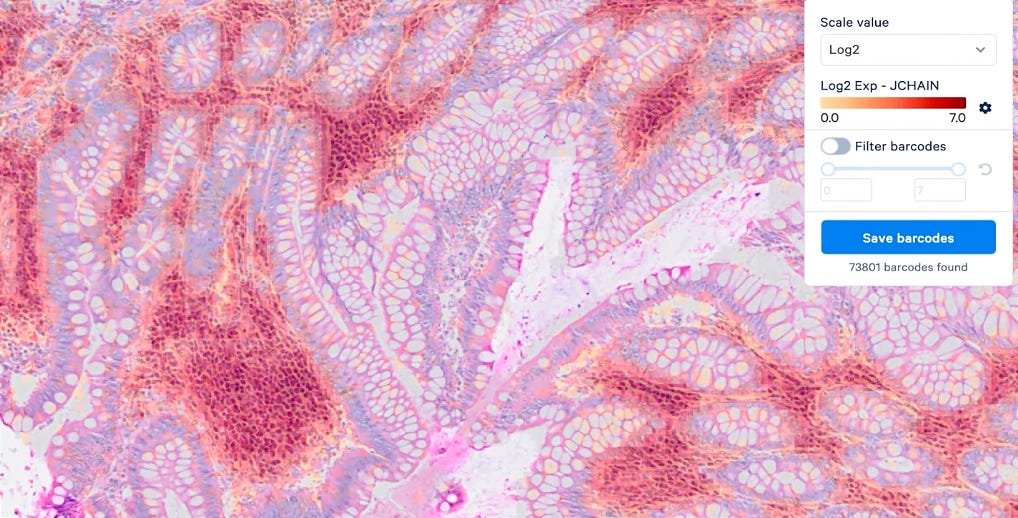
As a field, we’ve become incredibly skilled at measuring what biological systems are doing, thanks to next-generation sequencing — a topic I previously wrote about in Read, Write, Edit, Accelerate. With the rise of spatial sequencing we can even measure where these biological processes are occurring. Moving from two to three dimensions, in this manner, has led to a number of new possibilities. For example, we went from being able to identify what genes were differentially expressed in a tissue sample— a feat in and of itself— to now being able visualize both the localization of gene expression patterns and cell types within a tissue¹.

Spatially resolved expression of the JCHAIN gene in a tissue sample. Lighter yellow areas are regions with low expression, whereas dark red areas are regions with high expression (image source).

Consider what this stepwise change— from two to three dimensions— means in terms of impact. We can now see how the spatial distribution of immune cells can impact a tumors resistance to chemotherapy or how different regions of a tumor can have differing sensitivity to a given drug. Now, imagine the additional insights we could gain by moving beyond three dimensions, incorporating time in our measurements. When we explicitly consider time we can take full advantage of the unique temporal windows different omics platforms allow us to look through. Additionally, apparent contradictions between measurements— like in the case I opened this article with— disolve away, giving way to less convoluted chains of cause and effect.

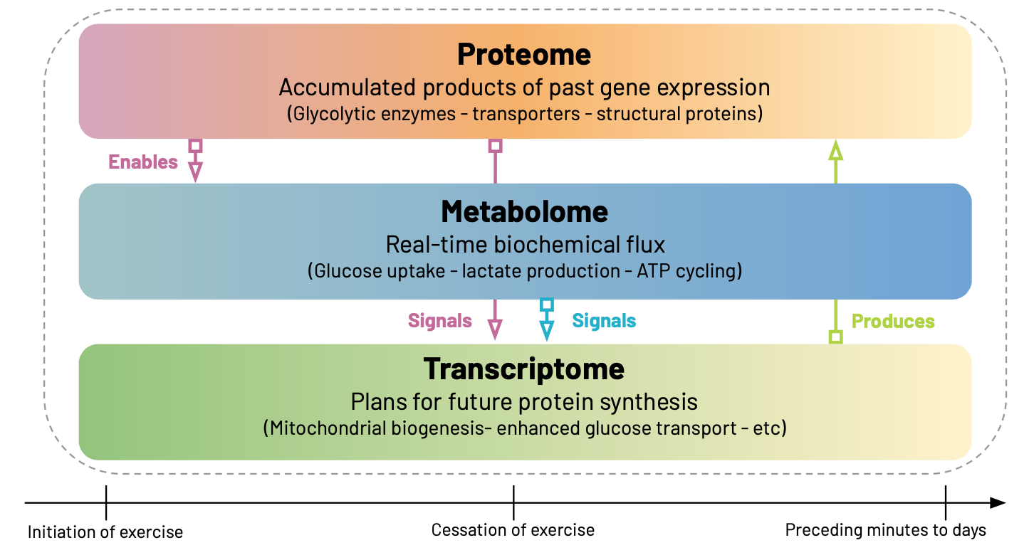
Every cell in our body exists in a temporal haze, carrying the accumulated products of past gene expression in its proteome, executing biochemical processes via its metabolome, and preparing for future changes through its transcriptome. Each of these "-omes” can be measured, through varying methodologies², providing us with different spatiotemporal perspectives on the same underlying system.

Consider what happens in skeletal muscle during high-intensity exercise. The proteins present at time t=0— glycolytic enzymes, transporters, and structural proteins accumulated over previous hours and days— determine how the cell can respond to the imposed energy demands. When exercise begins, this existing proteomic machinery drives the immediate metabolomic response: glucose uptake accelerates, lactate production increases, ATP cycling intensifies. The metabolome, at t=0, therefore reflects real-time biochemical flux— the actual work being performed by the proteins that are already in place.

But the cell doesn't just respond—it adapts. The metabolic perturbations triggered by exercise create a new intracellular environment rich in signaling molecules: elevated calcium, altered NAD+/NADH ratios, accumulating lactate, depleted glycogen. These metabolites don't just reflect current activity; they actively reshape gene expression by serving as cofactors, allosteric regulators, and epigenetic modifiers. Within minutes, transcription factors respond to these metabolic signals, initiating a gene expression program that will prepare the cell for future challenges.

Thus, the transcriptome, measured at t=0, captures the cells plans about what it will do next. Genes for mitochondrial biogenesis, enhanced glucose transport, and improved protein synthesis machinery become active—not because the cell needs these proteins right now (the acute stressor has come and gone) , but because the metabolic signals indicate it will need them in the coming hours and days.

This creates a temporal cascade where each omics layer both responds to the current state and influences future states. The proteins present now enable current metabolic responses, which generate signals that drive transcriptional changes, which produce proteins that will reshape future metabolic capacity. Understanding this "temporal architecture" is essential for making sense of multiomics data, especially when different measurements are captured at the same point in time, as in the case mentioned earlier³⁴.

The time-dependent nature of omics measurements can create both challenges and opportunities for cross-layer predictions. In theory, transcriptomic data should predict future proteomics data— after all, mRNA serves as a template for protein synthesis. Yet, anyone who has attempted such predictions inevitably encounters the notoriously poor correlation between mRNA and protein levels⁵ (see the footnote for specifics).

It’s clear that the protein-mRNA relationship is different for different genes and organisms, and that we shouldn’t expect it to be linear. However, I do suspect that the true correlation may be higher than those we frequently see reported, as most accounts compare mRNA levels and protein abundance measured simultaneously— essentially asking the question of whether the cell’s current plans (transcriptome) match its current capacity (proteome). This is like comparing a construction blueprint with an existing building and wondering why they don't match.

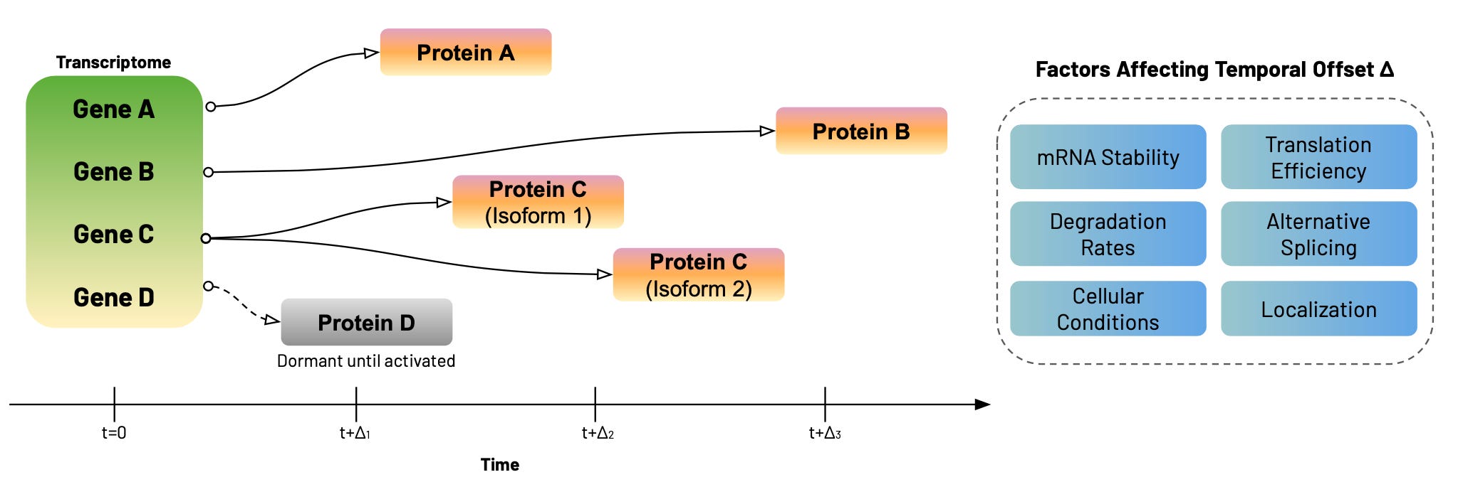
One solution is an intentional temporal offset in data collection. For example, transcriptomic measurements taken at t=0 can be compared to proteomic measurements taken at t+Δ, where Δ represents the time required for transcription, translation, and protein accumulation. Of course, the temporal offset Δ can vary dramatically— from minutes to days— depending on the specific gene and protein, mRNA stability, translation efficiency, post-translational modifications, and protein degradation rates. Some transcripts produce proteins within hours, while others remain dormant until specific cellular conditions activate translation. Alternative splicing can also generate multiple protein isoforms from a single gene, each with different temporal dynamics⁶.

This variability across cell types, individuals, and experimental conditions is exactly why we can't take it for granted that detecting gene expression guarantees protein production. The temporal disconnect between mRNA and protein levels isn't a measurement bug—it's a fundamental feature of cellular regulation that reveals the sophistication of biological control systems. In skeletal muscle, the Δ for muscle protein synthesis can be days, while in neurons synaptic proteins may only require hours to accumulate. One way to reconcile this could be to capture both transcriptomic and proteomic data at varying time points before and after a stimulus, then find the optimal lag where the former predicts the latter, or where causal relationships are strongest (using Granger causality, for example).

Another solution could be to incorporate epigenomic data, which could provide crucial context for these cross-layer predictions. A gene with high mRNA expression might seem poised for protein production, but if chromatin accessibility data shows repressive marks accumulating at its promoter, the transcriptional burst may be transient. Conversely, genes with moderate mRNA levels but strong activating epigenetic marks often show robust protein production in subsequent time points. In this way, the epigenome acts as a cellular memory system, encoding information about which transcriptional programs are likely to persist in a process that resembles hysteresis, which I wrote about in Bistability and Hysteresis in Biological Systems.

Multiomics data creates an analytical puzzle — every layer of biological information both influences and is influenced by every other layer, creating circular dependencies that obscure true causal relationships. Metabolites regulate gene expression, which in turn produces proteins that create metabolites. Proteins drive metabolite processes, which then modify protein activity. Biology is a mess. Without external reference points, we can easily get lost in recursive loops where cause cannot be separated from effect and correlation masquerades as causation.

Stimulus data breaks these loops by providing us with "temporal anchors" — specific perturbations that drive the biological system out of equilibrium and create traceable chains of cause-and-effect. Perhaps it’s my bias having come from the world of professional athletics before transitioning to computational biology, but to me exercise physiology provides us an ideal model — we can measure precise stimulus parameters (power output, duration, relative intensity) alongside the molecular responses they trigger across difference timescales, allowing us to deconvolute the underlying biological processes⁷.

When we map the exercise responses temporally, clear causal pathways emerge. The stimulus creates immediate demands on existing cellular capacity, visible in the metabolomic response. These metabolic changes activate signaling cascades that modify chromatin accessibility over minutes to hours, leading to transcriptional changes that drive proteomic adaptations over hours to days. Each step is both a response to the previous layer and a preparation for the next challenge.

Critically, this process creates adaptation—the next exercise bout encounters a system with altered baseline proteomic capacity, modified epigenetic priming, and different metabolic efficiency. The stimulus-response relationship itself evolves, which is why identical exercise protocols produce different physiological responses as training progresses. This adaptation represents biological learning encoded across multiple omics layers and time scales.

Traditional multiomics analyses treat each datatype as an independent matrix, potentially missing out on the rich temporal and causal relationships that connect genes to proteins to metabolites to phenotypes across different time scales. Knowledge graphs, on the other hand, excel at handling these temporal relationships because they can explicitly model the time-dependent connections between molecular entities⁸, providing a unified framework for integrating diverse data types and analytical outputs into a coherent, queryable representation of biological relationships.

Consider the typical workflow for analyzing different omics datasets. For transcriptomic, proteomic, and metabolomic data we could perform differential expression analysis to identify genes/proteins/metabolites that change between different conditions, functional enrichment analysis to understand affected biological processes and molecular functions, and co-expression analysis to find genes/proteins/metabolites that respond in tandem. Additionally, each datatype allows for novel analyses, like generating protein-protein interaction networks from differentially expressed proteins or performing isotope tracing to understand flux through metabolic networks.

Each of these analyses produces relationships that can be encoded in a knowledge graph. A differential expression analysis creates edges like gene -[upregulated_in]-> condition or gene -[downregulated_in]-> condition. Functional enrichment analysis produces pathway -[enriched_in]-> condition relationships. Co-expression analysis generates gene -[co_expressed_with]-> gene edges, often weighted by correlation strength. Similarly, protein-protein interaction data creates protein -[interacts_with]-> protein relationships, while cross-omics connections could emerge as gene -[encodes]-> protein edges, for example.

The power of this approach becomes apparent when you start integrating across analytical results. Instead of having separate lists of differentially expressed genes, altered proteins, and enriched pathways, you have a unified network where these results connect. This would allow you to do things like query for genes that (a) are upregulated in a condition, (b) encode proteins that show increased abundance, and (c) participate in pathways that are enriched. These integrated queries reveal biological coherence that's invisible when analyzing each omics layer independently.

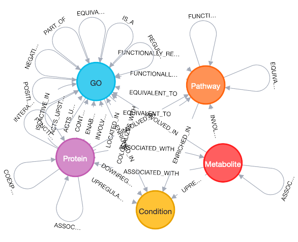
More importantly, knowledge graphs can incorporate the temporal relationships we've discussed. The gene-[encodes]-> protein relationship can be annotated with temporal metadata, creating gene@t=0-[encodes_with_delay]-> protein@t=2 relationships. Co-expression edges can be time-lagged, representing gene -[predicts_expression_of]-> gene relationships across time points. Pathway activities can be temporally ordered, showing how perturbations propagate through metabolic and signaling networks.

This structure enables queries impossible with traditional approaches. Instead of asking "which proteins correlate with differentially expressed genes in condition A?", we can ask "show me genes upregulated in condition A at t=1 hour that encode proteins showing increased abundance at t=6 hours, where both the genes and proteins are enriched in the same biological pathways." The knowledge graph naturally handles temporal offsets, finding meaningful connections across time and biological scale.

Even more powerfully, knowledge graphs can incorporate stimulus data— whether an exercise stimulus, drug dose, environmental change, or otherwise— as first-class entities⁹. For example, an exercise stimulus would become a node (rich with intensity, volume, and frequency metadata) that connects to immediate metabolomic changes, delayed transcriptomic responses, long-term phenotypic adaptations, and so forth. This would allow us to trace complete causal chains from environmental perturbations through the analytical results from each omics layer to phenotypic outcomes. However, I should note that while this capability is conceptually straightforward, I haven't seen robust implementations that handle stimulus integration effectively at scale. This represents a significant opportunity—one I've been eager to explore but haven't had the funding to pursue systematically.

I’ve spent considerable time working with biological knowledge graphs that integrate multiomic, phenotypic, and clinical symptom data, hence my focus on these types of approaches in this piece. However, I do want to acknowledge the fact that there are other viable frameworks for incorporating time into multiomics analyses. In fact, the honest truth is that we still don’t know which strategies will prove most effective in the long run. Traditional statistical approaches like time-lagged correlation and Granger causality remain powerful for many applications. Machine learning methods that treat temporal multi-omics as a dynamic system identification problem are showing promise as well. Even simple approaches—like carefully designed time-course experiments with targeted validation—can provide clear biological insights.

What strikes me most is how much we don't know about what we don't know. The temporal relationships I've described—the neat progression from transcriptomics to proteomics to metabolomics—may be oversimplified for many biological systems. Cells might operate with temporal dynamics that don't fit our current conceptual frameworks. The knowledge graph approach might reveal these unexpected patterns, or it might constrain our thinking in ways that prevent us from seeing more fundamental organizational principles. Time will tell.

It’s also possible that the most valuable outcome of building temporal multiomics knowledge graphs won't be the graphs themselves, but the process of attempting to build them. The technical challenges of data integration, the conceptual difficulties of modeling temporal relationships, and the practical problems of writing complex queries might force us to develop entirely new approaches to biological system analysis. The goal isn't to find the perfect solution immediately, but to start building something concrete enough to reveal what actually works and what doesn't. Let’s get working.

---

Did you enjoy this piece? If so, you may also want to check out other articles in Decoding Biology’s Bioinformatics & Biotechnology collection.

1. This has important implications for drug targeting. Through bulk proteomics (from a tumor tissue sample) we may find that a certain protein— say an antibody drug conjugate target— is highly expressed in the tumor. However, using spatial proteomics we may find that said protein is present deep within a solid tumor. This doesn’t mean it can’t be targeted, but it does mean there are certain physical and physiological barriers that need to be overcome since solid tumors can have abnormal vasculature and a dense extracellular matrix that impede drug delivery to the deeper regions. What originally appeared to be a slam dunk, from a drug target perspective, ends up looking a bit more complex through this newfound lens.

2. While beyond the scope of this article, it’s also important to consider how "multiomics" need not just refer to combining different omics types, like transcriptomics and proteomics. It can also mean combining different measurement technologies within a given "omics" subfield, allow us to get different perspectives on the same biological processes. For example, mass spectrometry (MS) and reverse phase protein arrays (RPPA) both allow us to measure protein abundance, but in very difference ways. MS gives us a relative measurement on a large number of proteins, whereas RPPA gives us an absolute measurement for a smaller, pre-defined, set of proteins. Two proteomics systems, two sets of complementary findings.

3. A key point here is that our knowledge of biology, without respect for how underlying measurement technologies work, can lead us astray. For example, we know that RNAs encode for proteins. As a result it’s natural to assume that proteomic measurements should reflect transcriptomic measurements, or that you can predict protein abundance from gene expression. However, when you consider the "temporal metadata" associated with each measurements — as discussed above— you can see how these relationships get blurred. Not to mention post translational modification, further impacting RNA-protein associations, as discussed by my friend Tommy Tang in a recent post.

4. The importance of understanding how measurement technologies work cannot be overestimated. Take mNIRS sensors: it’s common for people to interpret increases in SmO2 under high heat conditions as a shift in tissue oxygen balance from under to over supply. In reality, this is actually a signal artifact from increased cutaneous blood flow (for cooling), which begins to dominate the mNIRS signal on certain devices (generally older models). In fact, this interpretation is the opposite of what really occurs in the muscle — heat stress causes Hb to dissociate from oxygen more readily, leading to lower [true] SmO2 levels despite sensors potentially displaying the opposite pattern. Hence, the importance of understanding both the underlying biology and sensing modality to correctly interpret data.

5. I’ve seen the figure of r= 0.4-0.6 thrown around, but cannot find the exact source for this. However, there appears to be a good deal of organism specificity here, with R² values ranging from 0.2 to 0.87 (this would roughly equate to to an r of ~0.45 to 0.93) depending on whether we’re talking about bacteria, unicellular eukaryotes, or multicellular eukaryotes (like humans) — generally humans tend to fall on the lower range of R² values, as referenced in Global signatures of protein and mRNA expression levels. It also appears that Spearman correlations are often higher than Pearson, suggesting that the mRNA-protein abundance relationship is better described as monotonic vs linear.

6. Additionally, post-translational modifications, which dramatically alter protein function, localization, and stability in ways that transcriptomic data cannot predict.

7. There’s a great line in Human Cardiovascular Control, where Loring B. Rowell writes "Exercise, more than any other stress, taxes the regulatory ability of the cardiovascular system. The advantage to the investigator is that more is learned about how a system operates when it is forced to perform than when it is idle." This same concept can be applied to understanding biological processes and disease mechanisms in general. Rather than just studying pathological biological systems, we should also be studying biology at its opposite extreme. Notably, there are some groups doing this, like Variant Bio, and the Wu Tsai Human Performance Alliance.

8. For example, knowledge graphs allow us to move beyond static gene-protein relationships, representing dynamic pathways where genes at t=0 connect to proteins at t+2 hours, which connect to biological processes at t+4 hours, etc.

9. For stimulus integration, we could use wearable sensors and environmental monitoring systems, both of which generate rich time-series data that can be directly integrated with omics measurements.