Computational Modeling of Branched Pathway Systems

A DIY to Modeling Branched Pathway Systems With A Case Study In Metabolic Engneering

Enjoyed this piece? Show your support by tapping the “heart” ❤️ in the header above. It’s a small gesture that goes a long way in helping me understand what you value and in growing this newsletter. Thanks so much!

---

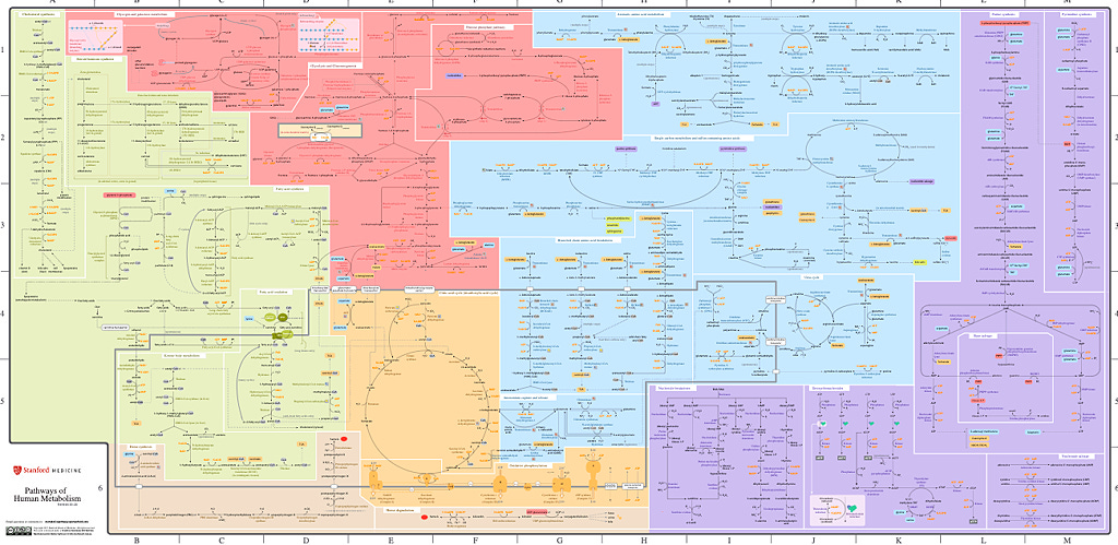
Cell metabolism is mind bogglingly complex. If you need convincing, take a look at Stanford’s Pathways of Human Metabolism Map— only rivaled in tortuousness by the streets in Boston.

Source

One of the things that always amazes me when looking at maps of cell metabolism is that few, if any, biochemical reactions proceed in isolation. Instead, they form complex networks where metabolites flow through interconnected pathways, creating branching structures with regulatory feedback loops.

Understanding these branching structures and systems, such that we can accuratley model them, opens up the door for all sorts of applications, ranging from metabolic engineering to drug development. In this article we’ll explore how computational modeling can help us decode these complex networks and how we can simulate their behavior. Let’s jump in!

The Biology of Branched Pathway Systems

Branched pathway systems are ubiquitous in biology, occurring anytime a common intermediate molecule serves as a starting point for multiple, distinct, chemical reactions (or pathways), leading to different end products¹.

Consider central carbon metabolism in microorganisms, which involves the enzymatic transformation of carbon sources— like glucose— into energy and various biosynthetic precursors needed for cell growth and function. For example, glucose enters glycolysis and from there the pathway quickly branches out, directing carbon flux toward different destinations including the pentose phosphate pathway, the TCA cycle, and amino acid biosynthesis.

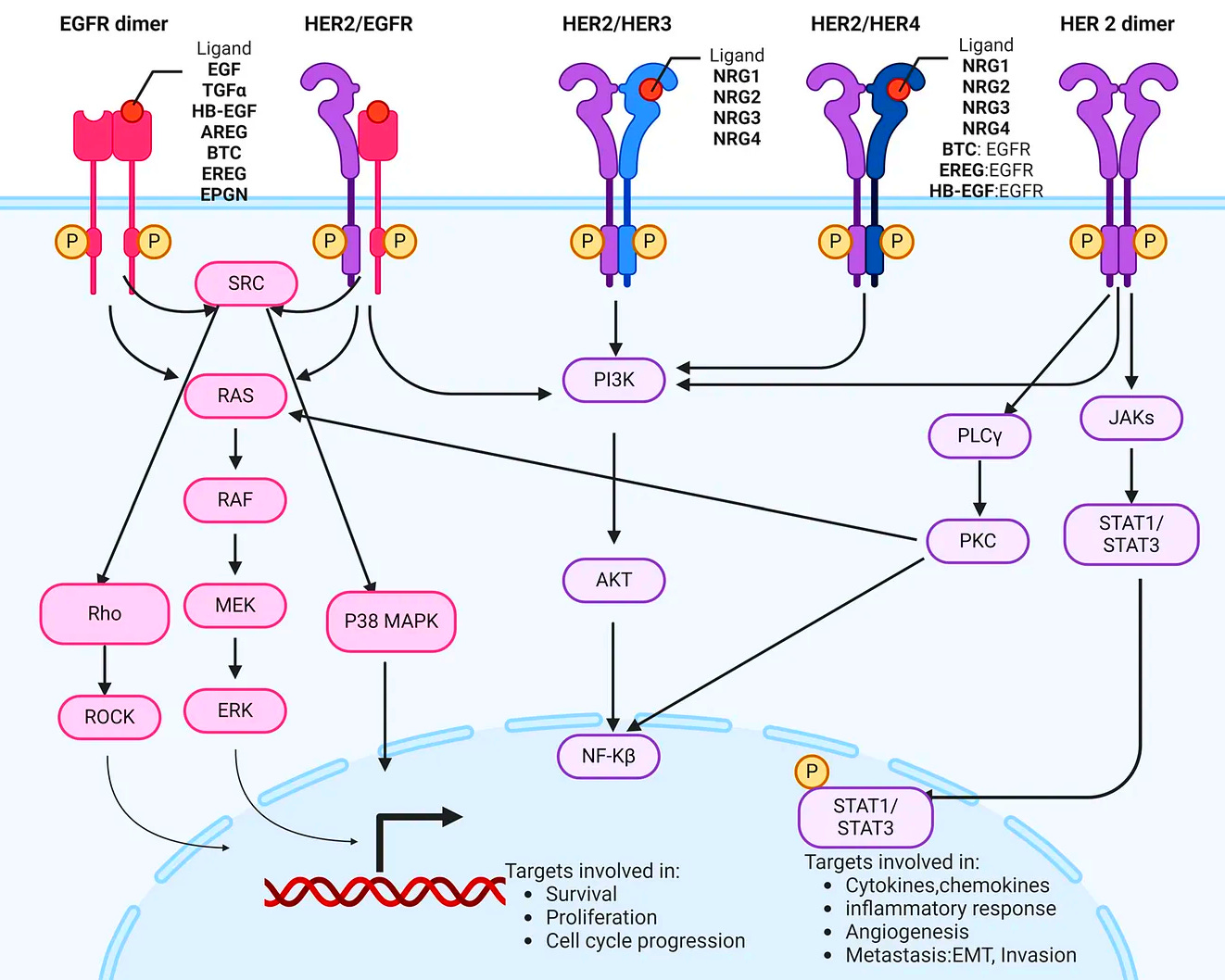
Similarly, signal transduction networks often feature branching cascades, where a single stimulus can trigger many different downstream events. Take the dimerization of HER2, which can simultaneously activate JAK, PLCγ, and PI3K, each in turn activating other proteins.

Source

The ubiquity of branched pathways systems in biology reflects their utility², and indeed they serve several important roles enabling cells to distribute resources efficiently based on current needs, maintain homeostasis through regulatory feedback, respond appropriately to environmental changes or stressors, and optimize energy utilization.

However, modeling branched pathway systems is not easy — in fact, their complexity creates many analytical challenges. When pathway X feeds into both pathways Y and Z, how does the cell "decide" how much flux goes in each direction? Additionally, how do feedback loops from other, distant, metabolites impact this distribution? These questions are difficult to answer through intuition alone, making computational modeling an essential tool — in the next section, we’ll explore this topic with a practical case study.

Mathematical Representations of Branched Pathways

Let's first visualize the branched pathway system we're working with, which represents a regulatory network with three main components (X1, X2, X3) and two external factors (X0 and X4). In this system, X0 is a constant input sources and X1 is the branch point metabolite that feeds into both X2 and X3.

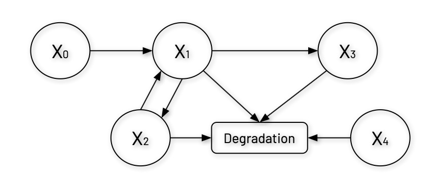
A notable feature of this system is the feedback loop between X1 and X2, where X1 promotes X2’s production, and X2 enhances X1’s production—this type of mutual positive regulation can lead to bistability³ or switch-like behavior in the system.

Additionally, each component in the system undergoes degradation, with X2’s degradation uniquely modulated by the external factor X4. This structure resembles regulatory networks common in biochemical processes and genetic circuits where the nonlinear interactions— represented by power functions in the equations below— allow for complex behaviors like threshold responses, oscillations, or multi-stability.

To create a mathematical representation of this system, we use ordinary differential equations (ODEs) that describe how the concentration of each metabolite changes over time:

\(\frac{dX_1}{dt} = y_{11}*X^{f110}_{0} * X^{f112}_{2} -y_{12} * X^{f121}_{1} - y_{13}*X^{f131}_{13}\)

\(\frac{dX_2}{dt} = y_{21}*X^{f211}_{1} - y_{22}*X^{f222}_{2} * X^{f224}_{4} \)

\(\frac{dX_3}{dt} = y_{31}*X^{f311}_{1} - y_{32}**X^{f323}_{3}\)

In these equations the y parameters (y11, y12, and so on) represent rate constants and the f parameters (f110, f112, etc) are kinetic orders or exponents that determine how strongly one metabolite affects another. This approach, which uses power-law expressions to represent the kinetics of each reaction, is known as Biochemical Systems Theory (BST) and allows for great flexibility in capturing complex regulatory relationships without requiring detailed enzyme mechanisms.

Python Implementation of Branched Pathway Systems

Now that we’ve covered mathematical representations of our branched pathway system, we can simulate the system using numerical methods⁴, as demonstrated in the code block below:

import numpy as np
from scipy.integrate import odeint
import matplotlib.pyplot as plt

# Define the branched pathway system (4.49)
def branched_pathway_system(q, t, X0, y11, y12, y13, y21, y22, y31, y32, f110, f112, f121, f131, f211, f222, f224, f311, f323, X4):
    X1, X2, X3 = q

    # Differential equations
    dX1dt = y11 * (X0 ** f110) * (X2 ** f112) - y12 * (X1 ** f121) - y13 * (X1 ** f131)
    dX2dt = y21 * (X1 ** f211) - y22 * (X2 ** f222) * (X4 ** f224)
    dX3dt = y31 * (X1 ** f311) - y32 * (X3 ** f323)

    return [dX1dt, dX2dt, dX3dt]

# Set the parameters as specified
X0, y11, y12, y13, y21, y22, y31, y32, f110, f112, f121, f131, f211, f222, f224, f311, f323 = 2, 2, 0.5, 1.5, 0.5, 0.4, 1.5, 2.4, 1, 0.6, 0.5, 0.9, 0.5, 0.5, 1, 0.9, 0.8

# Define initial values for X1, X2, and X3
initial_values = [1, 1, 1]

# Create time grid for the integration (0 to 100 seconds with 100 points)
time_grid = np.linspace(0, 100, 100)

# Explore different values of X4 between 0.1 and 4
X4_values = np.linspace(0.1, 4, 6)

# Set up the plot
plt.figure(figsize=(14, 8))

# Loop over different X4 values and solve the system
for i, X4 in enumerate(X4_values):
    # Solve the system using odeint
    solution = odeint(branched_pathway_system, initial_values, time_grid, args=(X0, y11, y12, y13, y21, y22, y31, y32, f110, f112, f121, f131, f211, f222, f224, f311, f323, X4))

    # Extract X1, X2, and X3 from the solution
    X1, X2, X3 = solution.T

    # Create a subplot for each value of X4
    plt.subplot(2, 3, i+1)  # 5 plots in a 3x2 grid
    plt.plot(time_grid, X1, label='X1', color='blue', lw=2)
    plt.plot(time_grid, X2, label='X2', color='red', lw=2)
    plt.plot(time_grid, X3, label='X3', color='green', lw=2)

    # Set title and labels for each plot
    plt.title(f'Trends for X1, X2, X3 with X4 = {X4:.2f}')
    plt.xlabel('Time')
    plt.ylabel('Concentration')
    plt.legend()
    plt.grid(True)

# Adjust layout to make sure plots don't overlap
plt.tight_layout()

# Show the plot
plt.show()

Which produces the following output:

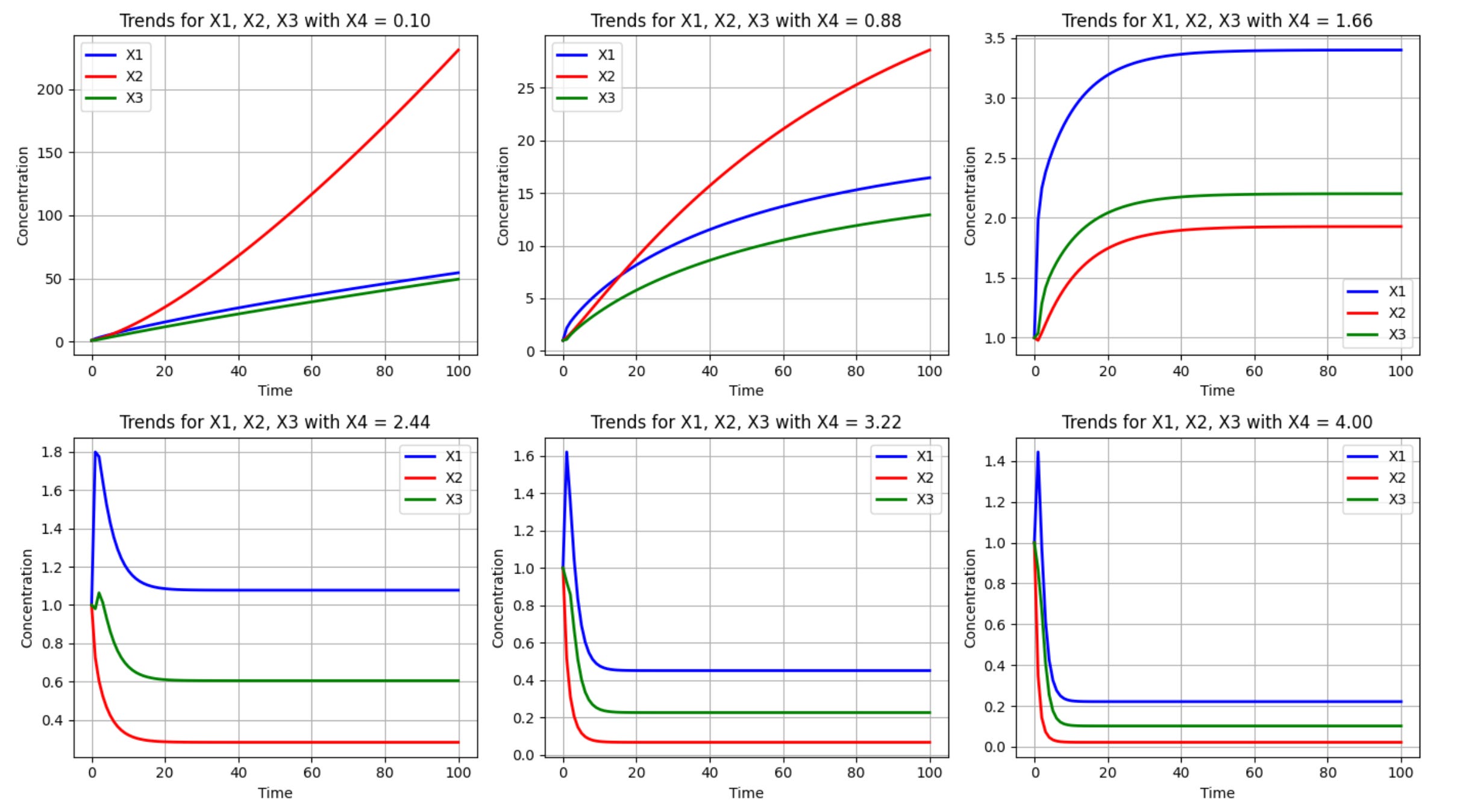
Let's analyze each equation in the code above:

• dX1dt: In the first equation, X1's rate of change (dX1dt) increases through production stimulated by both the input signal X0 and feedback from X2, while simultaneously being consumed through two separate pathways.

• dX2dt: The second equation shows X2 is synthesized directly from X1, but its degradation requires interaction with the external factor X4—a regulatory mechanism resembling cofactor-dependent processes in biological systems.

• dX3dt: The third equation demonstrates that X3 production depends solely on X1, with X3 undergoing its own independent degradation.

Additionally, by treating X4 as an adjustable parameter rather than a dynamic variable, this model framework allows for systematic investigation of how the system's behavior shifts under different environmental conditions or regulatory states, a standard approach in studying complex dynamic systems.

From Simulation to Insight

The true power of this computational approach lies in its ability to reveal system behaviors that might not be intuitive. For example, the simulations above reveal how varying levels of X3 affect all three metabolites (X1, X2, and X3) over time. Additionally, it captures both transient dynamics (how the system responds initially) and steady-state behaviors (where the system eventually settles). The simulation can also identify potential tipping points or thresholds where system behavior changes dramatically, as is the case with X4 values somewhere between 1.66 and 2.44.

These types of insights are useful for biotechnologists seeking to optimize metabolic pathways. For example, if X3 represents a desired product, the simulation might reveal the optimal level of X4 to maximize its production without disrupting cellular viability (represented by the balance of X1 and X2).

Additionally, these types of models and simulations have additional applictions in biotechnology including:

• Metabolic engineering: Predicting how genetic modifications might redirect flux toward valuable products

• Biopharmaceutical production: Optimizing culture conditions to enhance recombinant protein yields

• Synthetic biology: Designing artificial circuits with predictable behaviors

• Drug discovery: Understanding how potential therapeutics might affect metabolic regulation

Consider a biotech company engineering a microorganism to produce a valuable chemical. By constructing a mathematical model of the relevant pathways, they can simulate various genetic interventions in silico before investing in expensive lab work. This might reveal that inhibiting a competing pathway (analogous to reducing X2 in our model) would increase flux toward the desired product (represented by X3).

A Case Study in Metabolic Engineering

To make these abstract concepts more concrete, let’s consider a hypothetical application where our goal is to engineer E. coli to produce an amino acid derivative. In this system, X0 represents nutrient input to the system, X1 represents a branch-point metabolite like phosphoenolpyruvate (PEP), X2 is pyruvate, leading toward central metabolism, X3 is our target amino acid precursor, and X4 is glucose availability, which affects multiple pathways.

When simulating the effects of different glucose availabilities on this system we see that at low X4 (glucose) values X3 production is modest but consistent. At high X4 values we see an initial surge in X3, followed by a crash as regulatory mechanisms kick in to balance metabolism.

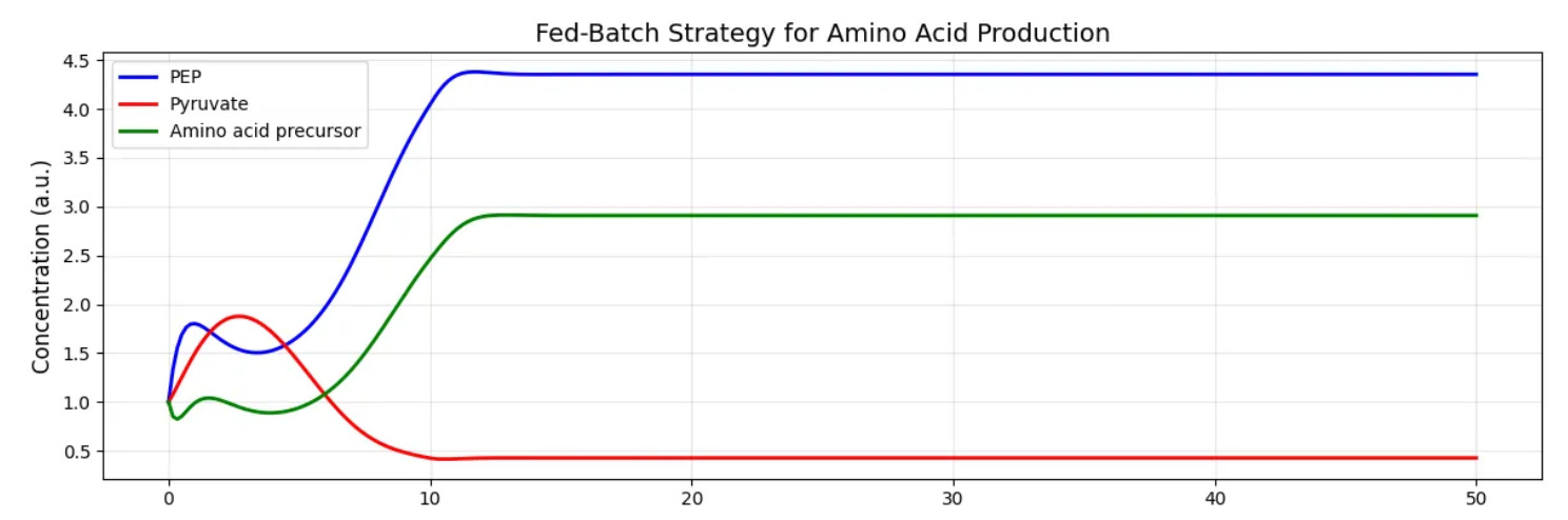
For a bioprocess engineer, this suggests that a fed-batch strategy, depicted above, with controlled glucose feeding might outperform both nutrient-rich and nutrient-poor conditions. The model provides a quantitative framework for optimizing this feeding strategy.

Real-World Challenges and Limitations

Modeling biolopgical systems is a powerful approach to understanding their workings, but there are several challgens we need to contend with:

1. Parameter estimation: real-world models can have dozens, or even hundreds, or parameters, which must be determined from experimental data. This is typically the most challenging aspect of ODE modeling in biology.

2. Model validation: Predictions must be validated against experimental data not used in parameter fitting.

3. Simplifications: All models, despite being useful, are simplifications. As such, they may not capture all biological complexities in a system.

4. Computational efficiency: As models grow larger, simulation becomes more computationally intensive.

Advanced techniques like sensitivity analysis, Bayesian parameter estimation, and model reduction strategies can help address these challenges, which will be the topic of a future Decoding Biology short.

---

Did you enjoy this piece? If so, you may also want to check out other Decoding Biology Shorts.

1. Branched pathway systems are a type of network structure that exhibits a "Y" shape, where a central node (or parent pathway) splits into two or more daughter pathways. These motifs are recognized as fundamental building blocks of larger, integrated signaling pathways and are found in various biological systems.

2. Branches pathway systems are one of many network motifs, which are reoccurring patterns that appears with statistically significant overrepresentation. In biological networks motifs are often evolutionarily conserved, meaning they are retained across different species due to their functional importance — ie, their conservation suggests the motif has been maintained by natural selection, preserving its role in the biological process it's involved in.

3. If you’re interested in learning more about this concept, you may enjoy an article I wrote previously, Bistability and Hysteresis in Biological Systems.

4. For a primer on numerical methods you can check out Numerical Methods in Systems Biology: From Euler to Runge-Kutta.