Unraveling Gene Co-Expression Networks: Insights into Transcriptional Regulation

A comprehensive guide to constructing and analyzing co-expression networks for biological discovery

Liked this piece? Show your support by tapping the “heart” ❤️ in the header above. It’s a small gesture that goes a long way in helping me understand what you value and in growing this newsletter. Thanks so much!

---

🧬 Unraveling Gene Co-Expression Networks: Insights into Transcriptional Regulation

Co-expression network analysis is a powerful approach for identifying groups of genes, referred to as "modules," that exhibit coordinated expression patterns across a dataset. These modules often represent functionally related genes, or sets of genes, that work together in shared biological pathways or cellular processes. By capturing patterns of gene activity, co-expression networks enable researchers to infer relationships between gene expression and biological traits or conditions. This makes them invaluable tools for uncovering the mechanisms driving disease progression, developmental processes, or responses to environmental changes.

One of the most widely adopted tools for constructing co-expression networks is Weighted Gene Co-expression Network Analysis (WGCNA). This method leverages pairwise correlations between gene expression levels to group genes into clusters, or modules, of tightly interconnected genes. Additionally, WGCNA highlights key genes within each module—known as hub genes—that are highly connected and often play pivotal regulatory roles.

This guide will introduce you to the principles of co-expression network analysis, walk you through constructing a co-expression network using WGCNA, and demonstrate how to identify key modules and hub genes associated with specific biological traits. Let’s get started!

🧬 How Does Co-Expression Network Analysis Differ from PPI Network Analysis?

As we’ve established, co-expression networks are a valuable tool for exploring transcriptional regulation and identifying coordinated patterns of gene expression. By grouping co-expressed genes into modules, researchers can uncover functionally related gene sets, correlate these modules with external traits, and pinpoint key regulatory genes. However, you might wonder how this approach differs from protein-protein interaction (PPI) network analysis—a topic I previously discussed in a tutorial titled From Genes to Networks: Uncovering Biological Insights through Protein-Protein Interactions.

While both approaches reveal relationships between biological entities, they do so at different levels of the biological hierarchy. Co-expression networks focus on transcriptional regulation, capturing the coordination of gene expression across samples. In contrast, PPI networks highlight the physical and functional interactions between proteins. Essentially, co-expression networks uncover the upstream regulatory relationships that drive gene expression, while PPI networks represent the downstream interactions between the proteins encoded by those genes.

Additionally, co-expression analysis provides a broader perspective, capturing genes that are functionally linked through shared expression patterns, even if the proteins they code for do not physically interact. For example, genes A, B, and C may form a co-expression module due to being regulated by a common transcription factor. While their proteins might eventually interact to form a functional complex, co-expression analysis focuses on their shared transcriptional regulation. In contrast, PPI networks explore the mechanistic relationships between the proteins themselve, offering a detailed view of how they collaborate physically to perform biological functions. Together, these two approaches provide a comprehensive understanding of biological systems, linking upstream regulation to downstream molecular mechanisms.

🧬 Constructing a Gene Co-Expression Network: Background and Approach

Now, in this section, I’m going to walk you through how to create a gene co-expression network. Before we dive into the practical steps, it’s important to first understand a key characteristic of this type of analysis. Unlike a protein-protein interaction (PPI) network, which requires a pre-generated list of differentially expressed genes (DEGs) as input, co-expression network analysis can be performed even if you only have sample data from a single condition. This makes co-expression analysis particularly versatile because it does not rely on prior differential expression analysis. Instead, it identifies patterns of shared expression among genes across your dataset, revealing modules of co-regulated genes that can offer unique insights into the regulatory framework of the biological condition under study.

For this tutorial, we’ll be using a file named countlist_5xFAD. This dataset includes gene expression data from 20 samples: 10 from 5xFAD mutant mice and 10 from wild-type (WT) control mice. This file is the output of a prior analysis I performed, exploring the similarities, differences, and overlapping features between three mutant mouse models of Alzheimer’s disease. While we are working with this specific dataset, the methods I’ll demonstrate can be applied to any dataset formatted as a CSV file where rows represent genes and columns represent samples, with only minor adjustments to the code.

Note: You can use this code to retrieve the 5xFAD mouse data (+ it's corresponding WT control data) from GEO, then clean and reformat it, so the resultant output file, countlist_5xFAD, is the same dataset I'm working with in this tutorial.

Notably, when you have a dataset with two experimental conditions, such as treatment and control, you have a choice in how you approach the co-expression analysis. You can either (1) combine all the data into a single analysis or (2) split the dataset by condition. Each approach has its merits depending on the research question you are addressing. A combined co-expression network analysis, which pools the data from both conditions, is typically used when the goal is to identify gene modules that are conserved across the conditions. These conserved modules often represent core biological processes or pathways that are not significantly altered by the experimental treatment (or in this case, disease progression).

On the other hand, separate co-expression analyses for the treatment and control groups are particularly useful if you are interested in comparing network structures and identifying condition-specific modules or hub genes. By analyzing each group independently, you can uncover gene modules that are unique to a specific condition. For instance, modules found only in the 5xFAD group may represent biological pathways disrupted in Alzheimer’s disease, while those unique to the WT group may reflect normal regulatory networks. This approach also allows you to compare network properties such as connectivity, hub gene identification, and module composition between the two groups, which can reveal critical differences in gene regulation under disease versus normal conditions.

In practice, researchers often start with a combined analysis to identify shared and genotype-associated modules. Afterward, they may refine their findings by performing group-specific analyses to further explore differences in network topology or module composition, which is the approach I’ll take in this tutorial. This stepwise approach—starting with a combined network and following up with group-specific networks—not only provides a broader perspective on the biological system but also ensures that subtle, condition-specific effects are not overlooked.

Now, in the code block below, we'll start by loading the libraries used in this tutorial, importing our data, and then calculating pairwise correlations between gene expression¹:

Note: You can find all of the code for this article in this GitHub repository.

Which produces the following output:

As you can see, the output above is a correlation matrix generated from our gene expression dataset using Spearman correlation. Note, that the matrix has the same set of genes in both the rows and columns (it's an 100x100 matrix). Each cell in the matrix represents the pairwise Spearman correlation between two genes based on their expression profiles across all samples. The diagonal values are all 1.0 because each gene is perfectly correlated with itself, and the off diagonal values represent the Spearman correlation coefficient between pairs of genes (the coefficient ranges from -1, which is a perfect negative correlation, to 1, which is a perfect positive correlation). Additionally, you'll note that some cells in the matrix show an NaN value. This occurs when at least one of the genes in a pair has constant expression across all samples (i.e., no variation) or when the gene has a very low (near zero) expression level across samples.

Now that we've created our correlation matrix, we'll use it as input to create a co-expression network, as demonstrated below:

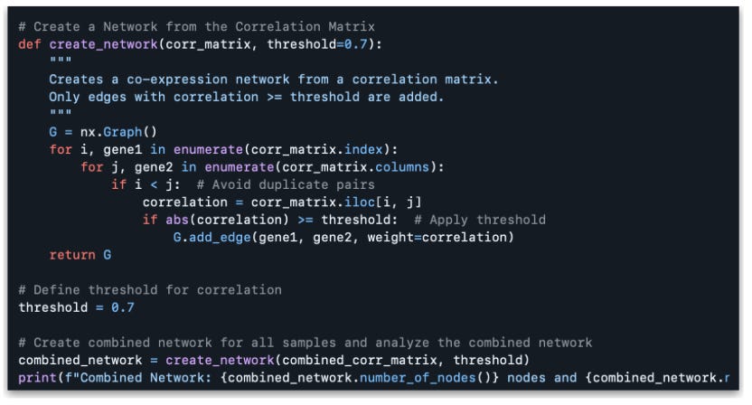
Which produces the following output:

Combined Network: 69 nodes and 583 edges

The output above tells us that our of the 100 gene in our dataset, 69 genes are included in our co-expression network and there are 586 edges (connections) between these genes. The reason we have 69 nodes in the network, and not 100, is that some genes may not have have a significant correlation (above threshold = 0.7) with any other genes, and as a result they are excluded from the network. The edges in our network represent pairwise relationships between genes based on their correlation. In other words, an edge exists between two genes if the absolute value of their correlation is greater than or equal to the threshold of 0.7.

Now, let's visualize the graph of our network along with the top 10 hub genes based on degree:

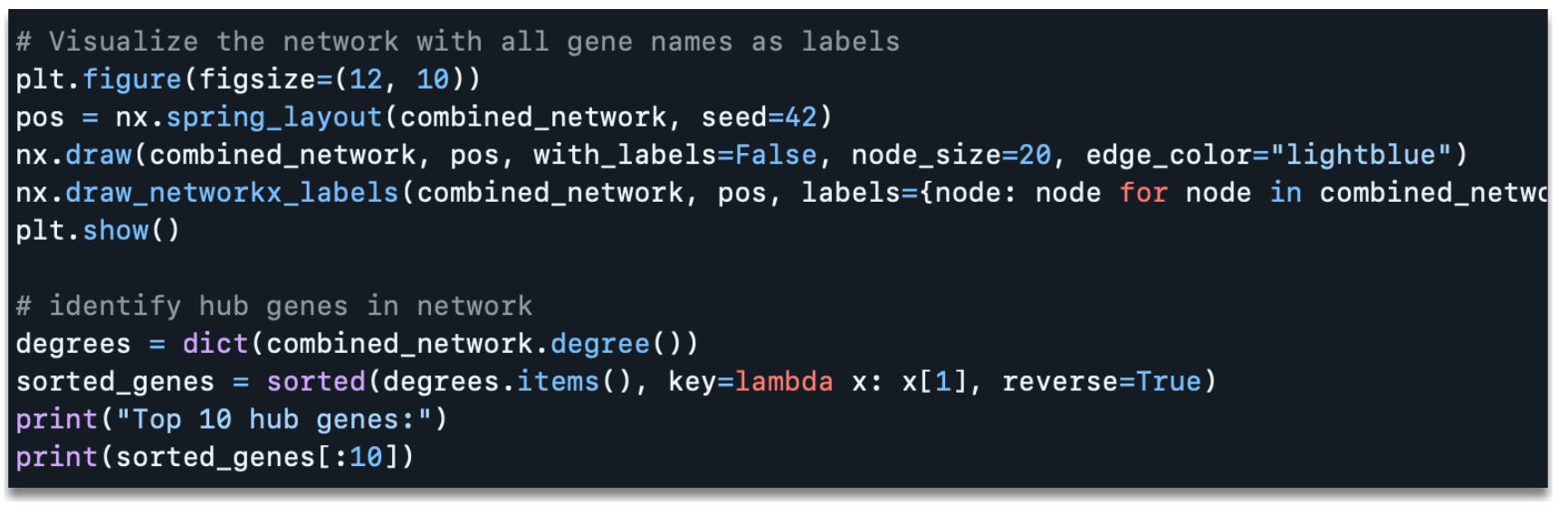
Which produces the following output:

Top 10 hub genes:[('Trappc10', 32), ('Gpr107', 32), ('Mkrn2', 31), ('Tfe3', 31), ('Brat1', 30), ('Dlat', 30), ('Hnrnpd', 30), ('Nalcn', 30), ('Dgke', 30), ('Cdh4', 29)]

In the figure above you can see the gene co-expression network with nodes labeled by gene name. Additionally, the code outputs the top 10 hub genes in the co-expression network, ranked by the degree (i.e., the number of connections) each gene has. For example, Trappc10 has 32 connections (edges), meaning it is co-expressed with 33 other genes are or above the threshold correlation of 0.7.

Using the degree to rank nodes is a simple and intuituve way to identify hub genes, as it reflects how many other genes a particular gene is co-expressed with above the threshold. However, we can also use more sophisticated metrics like degree centrality, clustering coefficient, betweenness centrality, and eigenvector centrality, which provide additional insights into the network structure and relationships between nodes, which we'll explore in the next section below.

🧬 Exploring Gene Co-Expression Network Connectivity

In the last sub-section, I introduced the metrics degree, degree centrality, clustering coefficient, betweenness centrality, and eigenvector centrality. Each of these metrics has it's own strengths and advantages, which I'll briefly outline below:

• Degree: The degree is the number of edges (connections) that a given node has, which reflects how many other genes a given gene is co-expressed with. This measurement provides a simple and fast measurement of network connectivity, despite it's simplicity.

• Degree Centrality: Degree centrality normalizes the degree of a node by dividing it by the maximum possible degree in the network. As a result, degree centrality gives a relative measure of how connected a node is compared to others in the network, making it a useful metric when comparing nodes in networks of different sizes.

• Clustering Coefficient: The clusterng coefficient of a node measures the connectivity of a node's neighbors, indicating how close they are to forming a complete (i.e. fully connected) graph. This measure is useful for understanding localized network structure and helps identify genes that are part of tightly connected modules.

• Betweeness Centrality: Betweeness centrality measures the frequency at which a node appears on the shortest paths between other nodes in the network, and as a result it identifies nodes that act as bridges or bottlenecks in the network. Nodes that rank highly on betweenness centrality may serve as critical regulators or mediators in the network.

• Eigenvector Centrality: This metric measures a node's influence in the network based on the influence of its neighbors. High eigenvector centrality indicates a gene is connected to many well-connected nodes, and as a result it identifies nodes with influence beyond their immediate connections (i.e. nodes with "global" influence).

For co-expression networks, degree, degree centrality, and clustering coefficient are most commonly used. However, if you're analyzing regulatory hubs or genes involved in key pathways, eigenvector or betweenness centrality could provide deeper insights. In the code below, we'll identify the top 10 hub genes baseds on degree centrality, clustering coefficient, betweeness centrality, and eigenvector centrality, and then we'll visualize sub-plots for each of these sets of hub genes:

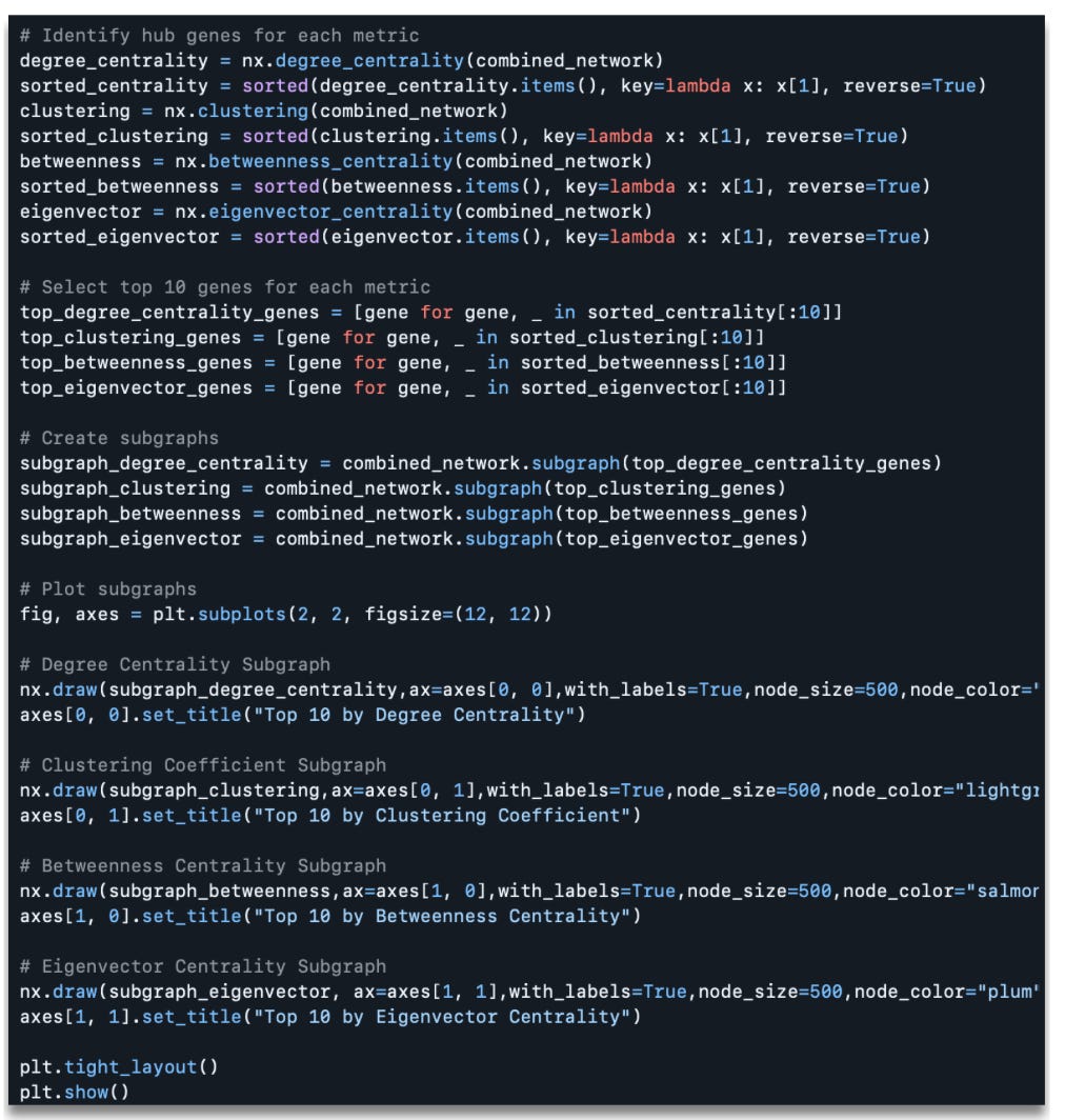
Which produces the following output:

As you can see in the figure above, analysis identified key genes in the co-expression network based on four centrality measures, each of which highlights different aspects of network topology, revealing the roles of these genes within the broader network structure.

• Top Genes By Degree Centrality: The genes with the highest degree centrality, such as Trappc10 and Gpr107, are highly connected within the network, indicating they may act as hubs coordinating interactions among other genes. These hubs are critical for the overall cohesion and robustness of the network.

• Top Genes by Clustering Coefficient: Several genes, including Cdc45, Fap, and Btbd17, had clustering coefficients of 1.0, suggesting they form tightly interconnected clusters. This implies that these genes might belong to highly specialized or functionally coherent modules within the network.

• Top Genes by Betweenness Centrality: Genes like Mkrn2, Comt, and Rtca exhibited high betweenness centrality, indicating their importance as bridges or intermediaries connecting different parts of the network. These genes could play a pivotal role in the flow of information or regulation between gene modules.

• Top Genes by Eigenvector Centrality: Genes such as Gpr107 and Trappc10 were ranked highest by eigenvector centrality, reflecting their influence in the network through their connections to other well-connected genes. These genes may be critical for maintaining the overall regulatory structure of the network.

Now that we've explored the combined network for our treatment (5xFAD mice) and control (corrsesponding WT mice) samples, we'll analyse the co-expression networks for each of these groups seperatley.

🧬 Exploring Gene Co-Expression Networks For Treatment and Control Samples (Separately)

As previously mentioned separate co-expression analyses for the treatment and control groups are particularly useful if you are interested in comparing network structures and identifying condition-specific modules or hub genes. By analyzing each group independently, you can uncover gene modules that are unique to a specific condition. For instance, modules found only in the 5xFAD group may represent biological pathways disrupted in Alzheimer’s disease, while those unique to the WT group may reflect normal regulatory networks. This approach also allows you to compare network properties such as connectivity, hub gene identification, and module composition between the two groups, which can reveal critical differences in gene regulation under disease versus normal conditions.

To continue exploring this tutorial, visiting my GitHub repository which includes the remaining analyses exploring gene co-expression networks for treatment and control samples separately, as well as all of the code used in this article:

1. I'm going to limit this analysis to the first 100 genes in my countlist_5xFAD file. This is to reduce computational load, as co-expression analysis can be very computationally expensive when using large datasets (and i'm using a personal machine to run the code in this tutorial).