The Biology Network

An introduction to static and dynamic network models and simulating metabolic pathways

An ask: If you liked this piece, I’d be grateful if you’d consider tapping the “heart” ❤️ in the header above. It helps me understand which pieces you like most and supports this newsletter’s growth. Thank you!

---

I recently revisited Yuri Lazebnik's essay, "Can a Biologist Fix a Radio?—Or, What I Learned While Studying Apoptosis," which critiques how biologists approach the study of complex systems. Lazebnik compares the way biologists investigate apoptosis (programmed cell death) to trying to fix a broken radio without fully understanding its components or how they interact. His essay highlights critical challenges in biological research, particularly the limitations of reductionism and the lack of system-wide integration.

Reductionism is the practice of breaking down systems into their component parts, which while useful for understanding the building blocks of biological systems in isolation often overlooks the complexity of interactions within a system. Lazebnik argues that knowing how parts work in isolation doesn’t necessarily lead to a full understanding of the whole, and in order to advance biological research we need to integrate our understanding of component parts into a broader more cohesive model.

As I pursue a PhD in computational biology, with a focus on systems biology, this essay resonates deeply with my work. In biological systems, proteins, genes, and metabolites don’t function in isolation but form vast, interconnected networks that drive processes like signaling pathways and metabolic reactions. These networks reveal how components influence each other, shaping their dynamics and functions. While traditional methods often focus on individual molecules or processes, tools like network analysis enables us to explore entire systems, uncovering coordinated behaviors and key players. This approach provides powerful insights into how biological systems function, adapt, or break down in response to factors like aging, disease, drugs, exercise, or environmental changes. In this article, we will explore the principles of network analysis, its ability to reveal hidden patterns in large-scale biological data, and its potential to deepen our understanding of complex systems beyond human intuition.

🧬 The Value of Static Network Models In a Dynamic World

Biological systems are inherently dynamic, with constant changes occurring at both macro- and microscopic scales. This raises a crucial question: Is it even worthwhile to study static networks that, by definition, do not change over time? The answer is yes, for several reasons. First, while biological networks do change over time, these changes are often gradual. As a result, static networks can accurately represent dynamic biological systems over short time scales. For example, consider studying gene expression changes following resistance training. Despite a robust hypertrophy stimulus, and increases in muscle protein synthesis, there will not be meaningful changes in muscle protein accretion or muscle cross-sectional area within a few minutes, hours, or even days, and as a result we can assume the system is static for the sake of simplified analysis.

Second, even in dynamic systems, assuming a temporarily static network can yield valuable insights. For instance, liver enzyme levels fluctuate over a lifetime and even within a 24-hour cycle. However, on the timescale of seconds or minutes—the focus of many models—these levels remain relatively constant, allowing us to perform static analyses to interrogate their function. Additionally, while a system may be dynamically changing at large, certain key features may remain static. For example, concentrations of metabolite pools might stay constant or in a steady state, even as regulatory signals fluctuate.

Beyond these conceptual reasons, there is also a practical advantage to studying static networks — the math involved in analyzing static networks are is far simpler when compared to dynamic systems. This simplicity allows even very large static networks to be analyzed with relative ease, whereas modeling similarly sized dynamic networks would be exceptionally challenging, let alone computationally expensive. Two aspects of static networks contribute to this simplicity¹.

🧬 Stratifying Static Network Models

The analysis of static networks can be categorized in various ways, beginning with the classification of networks based on whether they involve the flow of material or information. Networks that involve the flow of material, like metabolic networks, require precise accounting of masses, concentrations, and materials at each point (or node) in the network. For example, we know that the amount of products (i.e., metabolites) in metabolic network are directly proportional to the amount of substrate consumed to produce them, and as a result we need to accurately account for material flows through the system to ensure things add up properly.

Networks that involve the flow of information, by contrast, are concerned with the transmission of information. A prime example of this is a signaling pathway. The key difference between material- and information-based networks is that in the latter there is no accounting for inflow and outflows at a given node. In fact, the node that transmits information to another doesn’t “care” if the information ends up being used, or if it’s received by the second node. Additionally, signaling networks frequently involve all-or-nothing responses, like switching on gene expression in response to a stimulus (gene expression is either turned on in response to a signal or it isn’t), making mass accounting unnecessary.

Another way to stratify static networks is by the type of research activity they support, which can be broadly grouped into analysis focused research and construction/reconstruction focused research. Analysis focused research assumes that a network’s structure is already known and investigates the connectivity among components and their contributions to the system’s overall functioning. Construction/reconstruction, on the other hand attempts to infer the connectivity of unknown or poorly characterized networks from experimental observations, making it more challenging than analysis.

🧬 Interaction Graphs and Their Role in Network Analysis

When we study the structure of a network, the composition of the specific components becomes secondary. For example, it matters little whether the network is composed of proteins, sub-species, or populations. From a mathematical or computational perspective, these components are simply treated as nodes in the network and the connections between these nodes are called edges (edges are also referred to as links, interactions, or processes). Edges can be directed, undirected, bidirectional, and then an even contain regulatory features, as depicted in the image below.

(a) directed, (b) undirected, (c) bidirectional, (d) directed with regulatory features.

Taken together, nodes and edges form graphs, which are the principal representations of networks. Intuitivley, nodes in a network can only be connected by edges, and edges can only be connected with a node between them. For example, directed graphs are often used to represent transcriptional regulatory networks. Here, gene A might regulate gene B, but not vice versa, making the direction of the edges crucial. In contrast, protein-protein interaction networks are typically undirected since the interactions are mutual. Metabolic pathways can also be represented as graphs, where nodes are metabolite pools, and edges are chemical or enzymatic reactions. However, metabolic pathways also include regulatory features, which may require more complex representations, such as bipartite graphs, where two different types of nodes (e.g., metabolites and the locations where conversions occur) are represented, providing a more nuanced view of the network.

🧬 Introduction to Graph Theory: The Backbone of Network Analysis

Graph theory is a subdiscipline of math and computer science that provides the foundational tools for analyzing static network models, like those described above. Graph theory is primarily concerned with the properties of graphs, such as their connectivity, cycles of nodes and edges, the shortest path between nodes, and the most efficient way to partition a graph into unconnected subgraphs. In biological research, graph theory is primarily used to address questions about how a network is connected and what impact this connectivity has on the network's functionality. For example, graph theory is often used to characterize structural features such as the number and density of connections in different parts of a graph.

To understand the structure of a biological network, we can start with a graph composed of nodes and edges, like the two graphs depicted above. An important characteristic of a node is its degree, which represents the number of associated edges. For an undirected graph, the degree is simply the total number of edges at a given node. For example, in the left hand image above nodes N1, N2, N3, and N4 have degrees 4, 2, 2, and 4 respectively. In contrast, for directed graphs, it’s useful to define the in-degree and out-degree for a given node, which refers to the number of edges terminating or starting at a node, respectively. For example, in the right hand image above, node N1 has an in-degree of 3 and an out degree of 2, whereas node N4 has an in- and out-degree of 1.

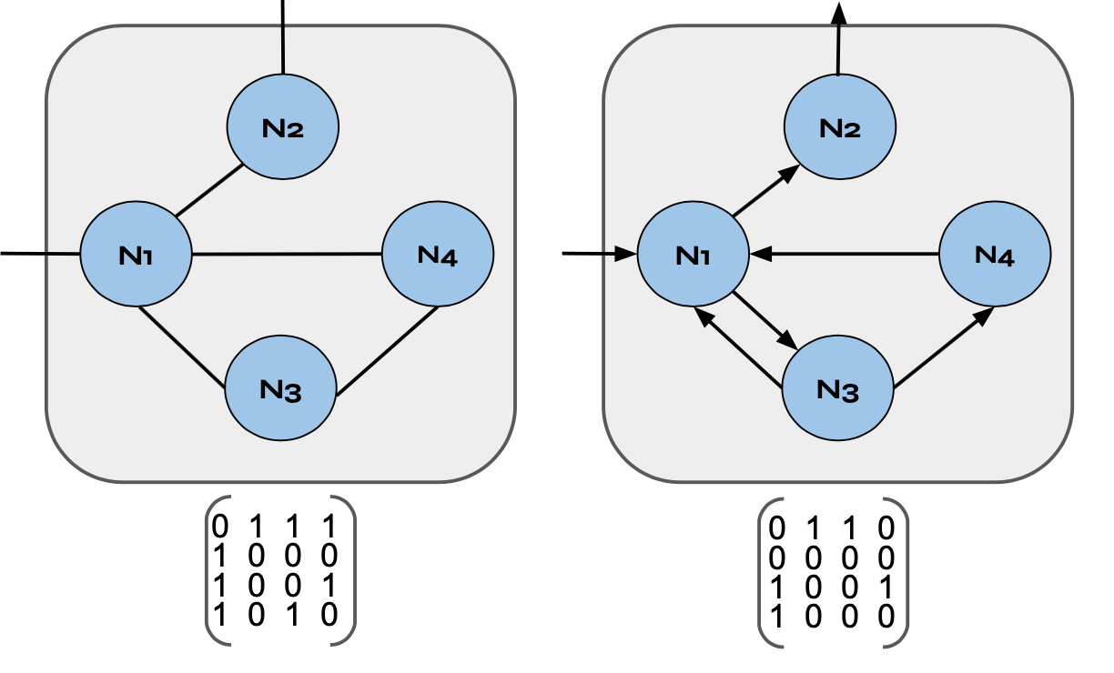
Another critical indicator of a graphs overall structure is its adjacency matrix, which uses 1s and 0s to indicate whether two nodes are connected, as demonstrated in the image above. In an undirected graph, edges are counted as two directed edges (one in each direction). For example, in the adjacency metric on the left we see that in the first column there is a 1 in the second, third, and fourth row, representing the fact that node N1 has a connection to node N2, N3, and N4. Additionally, we see that for node N2 (represented by column 2), there is a 1 in the first row since it is connected to node N1. However, in the adjacency matrix on the right 1’s only appear in the column for the node that is being connected to. For example, in the first column, representing node N1, we only have 1’s in rows three and four since nodes N3 and N4 are the only ones that have arrows pointing towards node N1.

Another important property to investigate is how edges are distributed within a given graph, which is assessed with a clustering coefficient metric, termed CN. The clustering coefficient quantified the density of edges associated with the neighborhood of a given node, and it ranges from 0 to 1 (with 1 indicating a fully connected node or clique). For undirected graphs, the clustering coefficient CN is 2e/k(k-1) where k represents the neighbors of a given node (ie. the number of nodes it is directly connected to) and e is the number of edges shared between a nodes neighbors. For directed graphs, the formula for CN is e/k(k-1). The image below contains an undirected (left) and directed (right) graph with a clustering coefficient calculated for each node.

In biological systems, graphs often exhibit high clustering coefficients compared to randomly connected graphs, which is a strong indication that biological systems are not the product of random organization. Additionally, as the size of a biological network increases, the average clustering coefficient among nodes decreases, suggesting that many biological networks consist of a high percentage of low-degree nodes with a small percent of highly connected nodes called hubs. This type of distribution where most nodes have a low degree and a few modes have a very high degree is called a scale-free network. An interesting feature of scale-free networks is that the shortest paths between randomly chosen nodes are significantly shorter than in random graphs. In random graphs, the average shortest distance is proportional to the logarithm of the number of nodes. In contrast, in scale-free networks, this distance is much smaller and increases more slowly as the network size grows. This property makes biological networks highly efficient in transmitting information across the system.

🧬 Analyzing Static Metabolic Networks

As previously mentioned, metabolic networks represent the flow of material through a system. More specifically, in a metabolic network, metabolite pools send and receive material, like organic compounds, which are represented by arrows connecting node to node. Additionally, in a metabolic network all materials flowing through the system need to be accounted for, and in many cases metabolic systems are modeled at a steady-state, which means the fluxes entering a given node have to be equal to the amount of fluxes leaving that node. As a result, steady-state metabolic networks can be “collapsed” into static networks that can be represented as graphs, like the one depicted below (note, the edges X are indicated with subscripts ‘to’ and ‘from’. For example, X12, represents the flow of material from N1 to N2).

If we assume that all edges in a metabolic network are unidirectional, as is the case in the image above where material flows from the left to right, the constraints imposed by the flow of material through the system can be reduced to mathematical relationships, which is called stoichiometry. For example, the stoichiometric equation for node N1 in the chart above is X01 = X12+X13 where’s the stoichiometric equation for node N3 is X13+X23 = X34. For a node like N2 we can dissect the bi-directional flux in edge X20 into two unidirectional fluxes toward and away from node N2, X02 and X20, allowing us to write the simple linear balance equation for node N2 as follows: X12+X02 = X23+X20.

These simple linear balance equations at each node is fully consistent with a dynamic metabolic systems model when we restrict the system to a steady state, as discussed above. To better understand why, let’s briefly suppose the system is not at a steady state. In this case, we can create differential equations that describe the network dynamics by equating change a node with the balances of materials entering and leaving the node. For example, a differential equation describing the flow of material through node N3 is dN3/dt = X13+X23 -X34, which means that the change in material through N3 over time is proportionate to the amount of material added to node N3 by edges X13 and X23, and the amount of material removed from node N3 by edge X34. In this differential equation, describing a dynamic system, X13, X23, and X34 are all time-dependent functions of metabolites whereas as a steady-state each flux takes on a fixed numerical value and as a result all of the derivatives in the system equal 0 (since there is no change over time). The result of assuming a steady state, and shifting to a static model, is that the system of differential equations describing the system are reduced to a system of simple algebraic equations. For example, in the case of node N3 the differential equation above becomes 0 = X13+X23-X34.

🧬 Bridging The Gap From Static To Dynamic Network Models

As previously mentioned, static network models offer valuable insights into the structure and interactions within biological systems, making it easier for researchers to analyze large networks and identify key components. By studying these static networks, we can better understand how biological systems are organized and how they function under stable conditions. However, biological systems are not static — they constantly change in response to internal and external stimuli and to truly capture the dynamic nature of these systems, static models can be expanded into dynamic models using ordinary differential equations (ODEs).

Dynamic models go beyond simply mapping the structure of a network. They account for how interactions between components change over time, allowing researchers to study the time-dependent behavior of a system. ODEs describe the rate of change for different elements within the network, providing a mathematical framework that can simulate how a system evolves.

Here’s why dynamic models offer significant advantages over static models:

• Time-Dependent Interactions: While static models provide a snapshot of interactions, dynamic models track how the strength and nature of these interactions change over time. This gives a more accurate representation of biological processes, such as fluctuating gene expression or enzyme activity in response to stimuli.

• Predicting System Behavior: Dynamic models can predict how a biological system will behave under different conditions. For example, ODEs can simulate how gene expression levels shift over time when exposed to a particular stimulus, offering valuable insights into potential outcomes of interventions.

• Capturing Feedback Loops: Many biological systems rely on complex feedback mechanisms to maintain balance, such as hormonal regulation or metabolic control. Dynamic models can incorporate these feedback loops, which are essential for understanding homeostasis and other self-regulatory processes.

Dynamic network models are especially useful in fields like biotechnology and drug development, where understanding how systems respond to interventions over time is crucial. By combining static network insights with ODE-based dynamic models, we can create more comprehensive frameworks that not only map out biological structures but also predict how these systems will behave, guiding experimental design and decision-making.

In the image below, you’ll find the metabolic network from the last section with differential equations describing the changes in metabolites concentrations at each node over time.

Now, we can model this metabolic network, and it’s fluxes over time, using the code below:

import numpy as np
from scipy.integrate import odeint
import matplotlib.pyplot as plt

# Set initial concentraions at nodes N1, N2, N3, N4
concentrations = [1.0, 1.0, 1.0, 1.0]

# Set fluxes at each node
fluxes = {"X_01": 1.0, "X_12": 1.0, "X_13": 1.0, "X_02": 1.0,"X_20": 1.0, "X_23": 1.0, "X_34":1.0, "X_40":1.0}

# create time grid
time_grid = np.linspace(0, 100, 100) # 0-100 seconds w/ 100 increments (1/sec)

# create function to model teh metabolic network
def metabolic_network(q, time_grid, X_01, X_12, X_13, X_02, X_20, X_23, X_34, X_40):
    N1, N2, N3, N4 = q

    # Differential equations describing fluxes at each node
    dN1dt = X_01 - (X_12*N1 + X_13*N1)
    dN2dt = (X_12*N1 + X_02) - (X_20*N2 + X_23*N2)
    dN3dt = (X_13*N1 + X_23*N2) - X_34*N3
    dN4dt = X_34*N3 - X_40*N4

    return dN1dt, dN2dt, dN3dt, dN4dt

# solve ordinary differential equations
solution = odeint(metabolic_network, concentrations, time_grid, args=(fluxes['X_01'], fluxes['X_12'], fluxes['X_13'], fluxes['X_02'], fluxes['X_20'], fluxes['X_23'], fluxes['X_34'], fluxes['X_40']))
N1, N2, N3, N4 = solution.T

# plot results
fig = plt.figure(facecolor='w')
ax = fig.add_subplot(facecolor='#dddddd', axisbelow=True)
ax.plot(time_grid, N1, alpha=1.0, lw=2, label='N1')
ax.plot(time_grid, N2, alpha=1.0, lw=2, label='N2')
ax.plot(time_grid, N3, alpha=1.0, lw=2, label='N3')
ax.plot(time_grid, N4, alpha=1.0, lw=2, label='N4')
ax.set_xlabel('Time')
ax.set_ylabel('Metabolite Concentrations Per Node')
ax.grid(True, which='major', c='w', lw=2, ls='-')
legend = ax.legend()
plt.show()

Which produces the following output:

Notably, in the code block above we set the starting concentrations at each node to the same initial value, and made all of the fluxes through nodes equal to one another. The result after executing the code is that the concentrations at nodes N3 and N4 rapidly increase while the concentrations at nodes N1 and N2 rapidly decrease (albeit at different rates) before the system reaches a new steady-state. However, we can experiment by changing the starting concentrations at each nodes, the rate of influx and efflux at a given node, or we can even add perturbations to the system to see how it responds. By doing so we can begin to gain a more comprehensive understanding of how integrated systems work, building progressively more sophisticated models for increasingly large static and dynamic metabolic networks.

---

🧬 Check Out BioloGPT, A Generative AI Model Designed to Answer Biological Questions.

Is there anything you didn’t understand from this article, topics you want to dig into more? Do you need help understanding the code block above, or debugging your own code to stimulate dynamic network models? If so, you may be interested in trying our BioloGPT, which is a sponsor of today’s post.

BioloGPT is engineered to be a highly-detailed, evidence-based, and skeptical AI committed to truth-seeking and answering biology questions as accurately as possible. It rigorously cites all used papers to ensure reliability, and can even generate novel hypothesis, code, art, and experiments. By citing relevant data and maintaining a critical, empirical stance, BioloGPT directly counters potential research biases such as positive result bias, framing bias, ideologies, censorship, scientific corruption, and industry influence.

1. There are two principle reasons why the math involved in static network analysis is far simpler than involved in analyzing dynamic network models. First, static networks do not change over time, and as a result the derivatives in the differential equations describing the network are all zero. As a result, the differential equations are tuned into simple linear algebraic equations, which are much easier to solve. Additionally, many static networks can be approximated as linear and as a result linear algebra can be used to analyze them — this is not true for many, or most, dynamic network models.