


Numerical Methods in Systems Biology: From Euler to Runge-Kutta
Modeling Gene Regulatory Networks Using Euler's Method and Fourth-Order Runge Kutta Methods.


Decoding Biology Shorts is a newsletter sharing tips, tricks, and lessons in bioinformatics. Enjoyed this piece? Show your support by tapping the ❤️ in the header above. Your small gesture goes a long way in helping me understand what resonates with you and in growing this newsletter. Thank you!
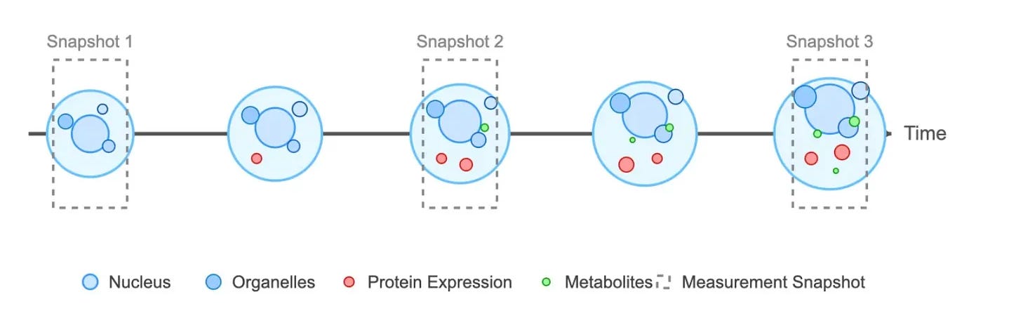
Cells are constantly humming with activity — genes switch on and off, protein concentrations rise and fall, and metabolites are produced, consumed, and shuttled back and forth. Understanding these dynamics presents a unique challenge as even the most advanced measurement technologies provide static snapshots at fixed points in time, leaving us wondering what’s really happening inside cells moment to moment. This is where simulations come in, providing us a lens, albeit an imperfect one, for understanding life at the smallest spatial scales.
One method for simulating molecular interactions is to turn them into systems of ordinary differential equations, which is a common technique used in systems biology. Once you’ve familiar with the methodology, writing systems of equations the process is relatively straight forward. However, as these systems of equations get larger, and more complex, we often run into the issue that they cannot be solved analytically. As a result, we have to use numerical methods1 to arrive at approximate solutions to these sets of equations.
One of the most intuitive numerical methods to work with is Euler’s method, which is named after the 18th century mathematician Leonhard Euler. In essence, Euler’s method provides a technique for solving ordinary differential equations by approximating solutions through small iterative steps, where the next value is computed using the current value and the derivative at that point. To use a biological example, imagine you’re tracking the concentration of a protein over time — if you know the current concentration and how fast it's changing, you can estimate the concentration a short time later by assuming the rate stays constant over that small interval2. Mathematically, Euler’s method states:
When tracking a protein’s concentration using Euler’s method, we start at our current concentration value and ask: "how fast is this changing right now?" Then we move a small distance in that direction. The formula tells us that the next concentration value equals our current concentration plus an adjustment term, which is calculated by multiplying how far forward in time we’re stepping (the step size, h) by how quickly the concentration is changing (ie, the derivative).
It's similar to estimating your location while hiking - if you know your current position and your current direction and speed, you can make a reasonable guess about where you'll be five minutes from now, assuming you maintain the same pace and direction. The limitation, of course, is that in reality, your path might curve or your speed might change, which is why Euler's method becomes less accurate over longer distances or in systems that change rapidly. This is particularly problematic in biological systems where concentrations can change dramatically within short timeframes. As a result, it’s often necessary to use more sophisticated numerical methods like the fourth-order Runge Kutta methods (RK4).
The Rk4 method, developed by Carl Runge and Martin Kutta in the early 1900’s, is a popular numerical technique for its simplicity and accuracy. It uses four slope estimates at each step to achieve a higher level of precision compared to simpler methods like Euler's method, as demonstrated below:
As you can see in the formulas above, the RK4 method uses four different “test steps” (k1, k2, k3, and k4), then combines them in a weighted average. This multi-sampling approach allows RK4 to "feel out" the changing landscape of the system, capturing how the rate of change itself changes within a single step, which is particularly valuable in biological systems where concentrations can accelerate or decelerate rapidly in response to regulatory feedback, ultimately resulting in more accurate predictions as compared to Euler’s method.
Now, in order to better understand the differences in performance between Euler’s method and the RK4 method, we’ll model a gene regulatory network and compare the results.
To give some biological context, gene regulatory networks represent how proteins control gene expression, often leading to complex dynamics. For this demonstration we’ll consider a simple two-gene circuit where protein A activates protein B, while protein B represses protein A, which is depicted and codified mathematically below:

The first equation in the image above, dA/dt, shows how protein A’s concentration changes over time: it increases through a term with k₁ (inhibited by protein B through a Hill function in the denominator) and decreases proportionally to its’ own concentration, γ₁A. The second equation, dB/dt, shows how protein B's concentration changes: it increases as a function of protein A's concentration (with parameter k₂) and decreases proportionally to its own concentration, γ₂B. These equations capture the activation-repression dynamics between the two proteins, where n represents the Hill coefficient that determines the steepness of the response curve.
Now, we’ll simulate this system of equations, modeling the dynamics of our gene regulatory network using both Euler’s method and the RK4. You can find my code used to generate the figures below here.

You’ll notice in the leftmost chart above that protein A and B’s concentrations show noticeable variations with different step sizes (ie, h values), especially in the oscillatory regions of the protein’s dynamics. The reason for this is that Euler’s method makes simple linear approximations at each step, whereas the RK4 method produces much more consistent results across different step sizes because it samples the rates of change at multiple points within each step. Additionally, Euler’s method becomes unstable with larger step sizes (h>=0.5), which produces ratification oscillations, or numerical instabilities3. This is particularly problematic for systems where protein production and degradation occur at different timescales.
The differences in performance between Euler’s method and the Runge-Kutta method have serious biological implications. Consider how Euler’s method may predict incorrect proteins levels, especially at peaks and troughs of oscillations. This could lead to incorrect conclusions about maximum protein expression levels when modeling real systems. Additionally, Euler's method may incorrectly identify the timing of state transitions or miscalculate periods of oscillations in biological systems.
To put these findings in a broader context, the choice of numerical method isn't just a computational concern—it directly impacts our understanding of biological reality. When modeling cellular processes like circadian rhythms, cell division cycles, or immune responses, these inaccuracies could lead to fundamentally flawed predictions about system behavior. A miscalculation in protein concentration dynamics might suggest an incorrect therapeutic window for drug delivery or misrepresent how quickly a cell responds to environmental stimuli. Furthermore, as we move toward whole-cell modeling and increasingly complex multi-scale simulations, the compounding effects of numerical errors become even more significant. What begins as small deviations in protein concentrations can cascade into large-scale prediction errors about cellular phenotypes or tissue-level behaviors.
While RK4 offers significant improvements over Euler's method, it represents just one point along the spectrum of numerical approaches. Depending on the biological system being modeled, you might need to consider adaptive step-size methods, implicit solvers for stiff systems, or stochastic simulation algorithms that account for the inherent randomness in biological processes.
Ultimately, the art of biological modeling requires balancing computational efficiency with biological accuracy. Understanding the strengths and limitations of different numerical methods isn't just a mathematical exercise—it's essential for building reliable computational models that can meaningfully advance our understanding of life at the smallest scales.
Did you enjoy this piece? If so, you may also want to check out other Decoding Biology Shorts.
Numerical methods are techniques used to find approximate solutions to mathematical problems, particularly when exact solutions are difficult or impossible to obtain analytically. If you’re interested in learning more about common numerical methods you can check out Systems Biology & Metabolic Engineering section of my Bioinformatics Toolkit.
Intuitively, you can imagine how using smaller step sizes in Euler’s method generally leads to a more accurate approximations of the solution to a differential equation. However, there's a trade-off as smaller step sizes require more calculations, which can increase computation time. As a result, Euler’s method isn’t always the most practical, or accurate, numerical method for solving complex problems.
Like Euler’s method, RK4’s accuracy improves with smaller step sizes. However, RK4 maintains greater stability with larger steps, making is more robust for modeling systems with production and degradation rates occur on different timescales.