


From Genes to Networks: Uncovering Biological Insights through Protein-Protein Interactions
Mapping DEGs to PPI Networks, Identifying Network Hubs and Highly Connected Proteins, and Simulating Genetic Circuits. An End-to-End DIY Guide


Liked this piece? Show your support by tapping the “heart” ❤️ in the header above. It’s a small gesture that goes a long way in helping me understand what you value and in growing this newsletter. Thanks so much!
🧬 From Genes to Networks: Uncovering Biological Insights through Protein-Protein Interactions
Differential expression analysis is a cornerstone of bioinformatics, enabling researchers to identify differentially expressed genes (DEGs) that exhibit significant changes in expression between varying experimental conditions. By comparing gene expression profiles between control and treatment groups, we can uncover molecular mechanisms underlying biological processes, disease states, or treatment responses. One valuable way to further explore these findings is by mapping differentially expressed genes to a protein-protein interaction (PPI) network.
A PPI network is a powerful tool for examining the relationships between proteins within a biological system. Unlike genes, which typically act independently, proteins interact with each other to perform essential cellular functions. These interactions are critical for maintaining biological processes, and when disrupted, they can contribute to disease states.
By mapping differentially expressed genes (DEGs) to a PPI network, we can gain deeper insights into how the proteins encoded by these genes are interconnected and how changes in gene expression translate into broader biological effects. In this article, you’ll learn what PPI network are, how to map DEGS to PPI networks and identify “hubs” in the network, and how to simulate genetic circuits using this information. Let’s dive in!
🧬 What Can We Learn From PPI Networks?
As previously discussed, a Protein-Protein Interaction (PPI) network is a powerful tool for examining the relationships between proteins within a biological system. By mapping differentially expressed genes (DEGs) to a PPI network, we can visualize how the proteins they encode interact with one another, providing insights into the molecular mechanisms underlying the observed phenotype.
Additionally, analyzing the PPI network allows us to identify biological pathways and cellular processes that are significantly influenced by the experimental conditions. These interactions often highlight key pathways involved in disease progression, cellular stress responses, or signaling cascades. Using clustering analysis, we can uncover tightly-knit protein modules, which may be enriched for specific biological functions relevant to the study. For example, proteins within a cluster might be involved in a shared signaling pathway or cellular response, pinpointing areas for deeper exploration.
Furthemore, one of the most valuable aspects of PPI network analysis is the identification of protein hubs, which are highly connected proteins that play central roles in the network. These hubs are essential for maintaining network stability and coordinating multiple cellular processes. Additionally, hub proteins are often involved in critical cellular functions, such as regulating gene expression or controlling signal transduction. Due to their centrality in biological processes, hub proteins are prime candidates for experimental validation, as they may drive pivotal events in disease progression or response to treatment.
🧬 Mapping DEGs to A PPI Network
Now, in this sub-section I'm going to show you how to map DEGs to a PPI network. For this demonstration I'm going to use a file named deg_5xFAD, which is an output file from a previous analysis I performed exploring the similarities, differences, and overlapping features between three mutant mouse models of Alzheimer’s disease. However, you can use any CSV file containing differentially expressed genes, with only minor modifications to the code below:
All code from this article can be found in the following GitHub repository.

Which produces the following output:

The figure above illustrates how the up- and down-regulated genes in our experimental system, collectively referred to as DEGs, are mapped to their corresponding protein products. Ideally, all DEGs in our CSV file should map to the PPI (protein-protein interaction) network, provided the corresponding protein interactions for each gene exist in the database we are using.
Mapping DEGs to a PPI network allows us to focus on the proteins encoded by these genes and understand how they interact within a biological system. For instance, if a gene like Slc22a18 is present in your DEG list, it encodes a specific protein. That protein might interact with other proteins in the PPI network. By mapping DEGs to the network, we can visualize and analyze these connections, offering deeper insights into the molecular interactions underlying our experimental system.
However, upon closer inspection, we may notice that some proteins in the PPI network are not directly encoded by genes in our DEG list. This discrepancy arises because the differentially expressed genes in our analysis represent only a subset of the proteins involved in the biological processes we are studying. A PPI network, on the other hand, includes all proteins (not just DEGs) and their interactions. This means that even proteins not differentially expressed may still appear in the network if they interact with DEGs. These non-DEG proteins could play essential roles as intermediaries between DEGs, participate in compensatory or regulatory mechanisms, or contribute to broader network stability and function.
To better understand the structure of our PPI network, we can begin by examining key network properties, such as the number of nodes, edges, and overall network density. These metrics provide an overview of the network’s connectivity and complexity, which we’ll explore with the code below:

Which produces the output:
Number of nodes: 263
Number of edges: 1059
Network density: 0.030737526485356863
To interpret the results of our network analysis, let's break down the key metrics in detail:
Nodes: Our network contains 263 nodes, representing the unique proteins present in the protein-protein interaction (PPI) network. These nodes correspond to proteins encoded by the differentially expressed genes (DEGs) in our dataset. However, it's worth noting that our DEG list initially contained 444 genes, meaning not all DEGs could be mapped to the PPI network. This discrepancy could arise for several reasons. For example, some DEGs may not have corresponding protein interaction data available in the PPI database. Alternativley, the analysis settings may filter out low-confidence interactions or proteins with weak evidence of interaction, highlighting the importance of understanding the limitations of the PPI database and the filtering criteria applied during network construction.
Edges: The network has 1059 edges, which represent the interactions (connections) between the proteins in the network. A higher number of edges relative to nodes suggests a more interconnected network, where many proteins interact with multiple partners. With 263 nodes and 1059 edges, our network exhibits a relatively complex interaction pattern. This indicates that the proteins encoded by the DEGs are part of a broad array of interconnected cellular processes, consistent with the intricate molecular interactions underlying biological systems.
Network Density: The network density is 0.0307, which measures the proportion of realized edges compared to the total possible edges. In this case, only about 3.07% of all potential connections are present. While 1059 edges may seem substantial, the theoretical maximum number of edges for a network with 263 nodes is (263 × 262) / 2 = 34,453. The low density reflects that most proteins in the network do not interact directly with each other, leading to a sparsely connected network.
In the context of the 5xFAD mouse model, a lower network density and sparse connectivity are biologically meaningful. This model is designed to study Alzheimer’s disease, a specific pathological condition with targeted biological pathways and cellular processes. Thus, the DEGS in our CSV file are likely associated with key disease-relevant pathways, rather than being broadly expressed across all cellular functions. As a result, the corresponding PPI network reflects the focused nature of these interactions.
While we’ve established that our network is sparse, the next question is whether it is fragmented. A fragmented network would contain multiple disconnected components, meaning there are proteins or groups of proteins that do not interact with the rest of the network. Identifying whether the network is fragmented will help us determine how cohesive the identified interactions are and whether the DEGs form a unified system or several distinct sub-networks. Let’s explore this further:
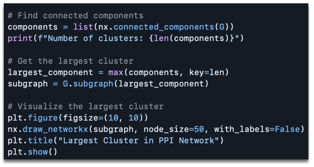
Which produces the output:
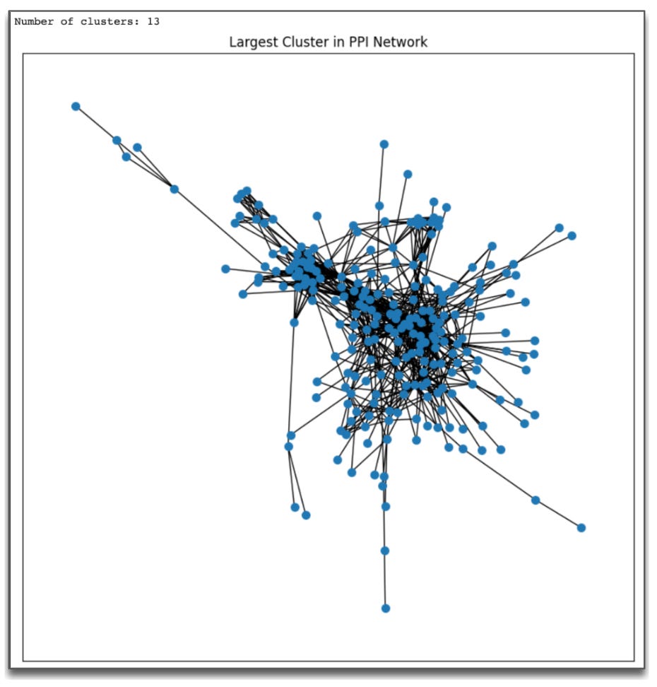
Using the code above, we observe 13 distinct clusters within our PPI network. The presence of clusters in a PPI network is a strong indication of functional organization. Proteins that cluster together tend to participate in similar biological pathways, such as signaling cascades, metabolic processes, or cellular responses. For instance, one cluster might represent proteins involved in neuroinflammation, while another might include proteins related to synaptic signaling or oxidative stress, all of which are relevant to Alzheimer’s disease in the 5xFAD mouse model. Clustering allows us to pinpoint these specific processes and focus on the biological mechanisms most impacted by the experimental condition.
Additionally, the combination of a sparse network and multiple clusters provides additional insights. While the overall network is not densely interconnected (as reflected by the low network density), the clusters indicate that certain subsets of proteins are tightly connected. This means that while the DEGs may not form a globally interconnected network, they do organize into biologically meaningful groupings. These clusters are likely to represent key processes relevant to the disease, even if they do not interact extensively with one another across the network.
To further understand the importance of these clusters and the overall connectivity of our PPI network, we can delve into additional metrics such as degree centrality, betweenness centrality, and the clustering coefficients, which can help uncover key proteins and interactions within the clusters that are most relevant to the biological processes under investigation.
🧬 Exploring the Connectivity of A PPI Network
Network analysis metrics such as degree centrality, betweenness centrality, and clustering coefficient each offer unique perspectives on the connectivity and significance of individual proteins within a protein-protein interaction (PPI) network. Together, these measures help identify key players, mediators, and tightly-knit communities within the network, providing critical insights into the biological mechanisms underlying your experimental system. In the code below, we'll identify the top 10 proteins based on each of these metrics:
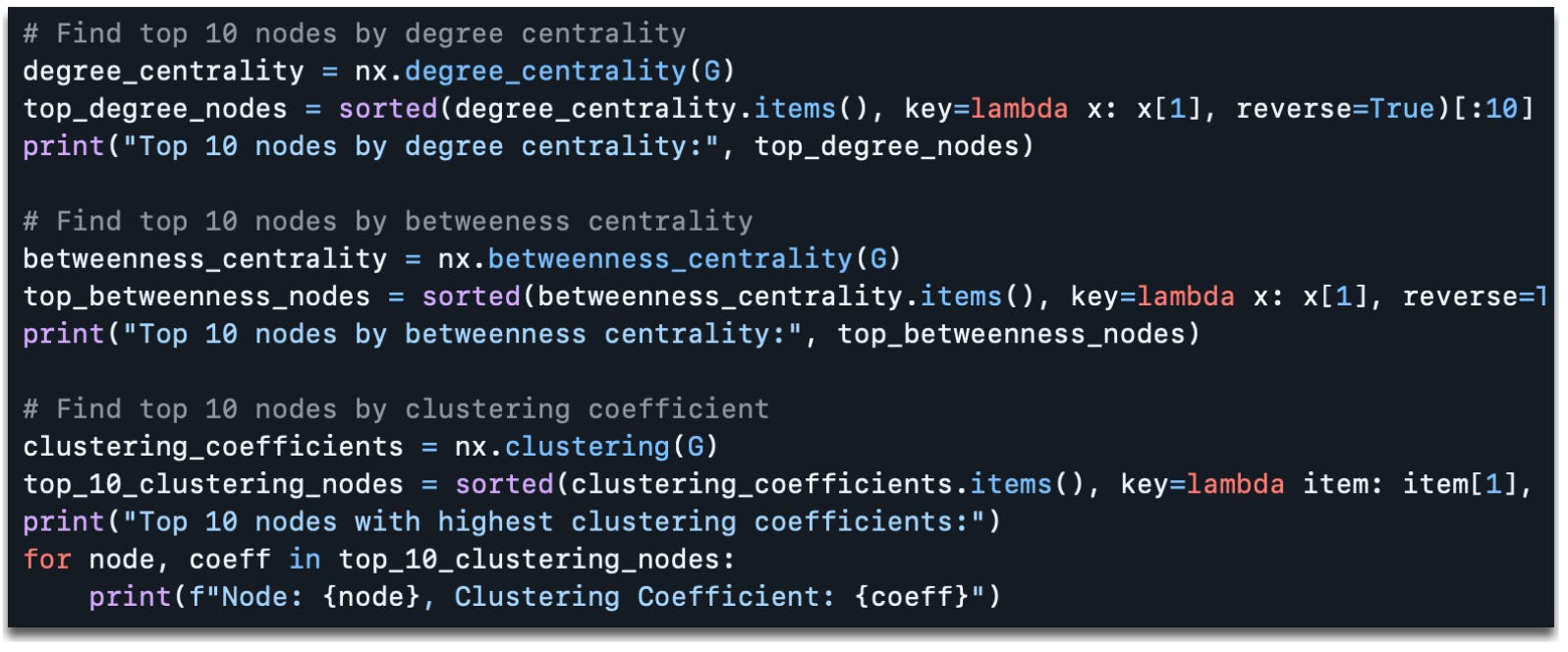
Which produces the following output:
Top 10 nodes by degree centrality: [('Ptprc', 0.17938931297709923), ('Stat1', 0.15267175572519084), ('Cd86', 0.13740458015267176), ('Cxcl10', 0.1297709923664122), ('Csf1r', 0.12595419847328243), ('Irf7', 0.12213740458015267), ('Fcgr3', 0.11832061068702289), ('Tyrobp', 0.11450381679389313), ('Itgax', 0.11068702290076335), ('Ifit3', 0.11068702290076335)]

Top 10 nodes by betweenness centrality: [('Ptprc', 0.1294639736031357), ('Stat1', 0.08417468655499585), ('Cxcl10', 0.07267041294833336), ('Csf1r', 0.06729005320986972), ('Vav1', 0.06172100839502038), ('Itgb2', 0.06097480610098475), ('Tyrobp', 0.05926978612196263), ('Cd86', 0.05711683901197365), ('Icam1', 0.05256193777917538), ('Nckap1l', 0.04846530517616378)]

Top 10 nodes with highest clustering coefficients:
Node: Selplg, Clustering Coefficient: 1.0
Node: F11r, Clustering Coefficient: 1.0
Node: Lyl1, Clustering Coefficient: 1.0
Node: Il3ra, Clustering Coefficient: 1.0
Node: Fyb, Clustering Coefficient: 1.0
Node: Tec, Clustering Coefficient: 1.0
Node: Sh3bp2, Clustering Coefficient: 1.0
Node: Cyba, Clustering Coefficient: 1.0
Node: Ncf2, Clustering Coefficient: 1.0
Node: Oas1g, Clustering Coefficient: 1.0
Degree centrality measures the number of direct connections (edges) a node has. In the context of a PPI network, nodes with high degree centrality represent "hubs"—proteins that interact with many others. These hubs often play central roles in cellular functions, acting as key regulators or drivers of biological processes. For example, the protein Ptprc, which ranks highest in degree centrality in this network, interacts with numerous other proteins, suggesting it may serve as a critical hub influencing multiple pathways. Other top-ranked proteins like Stat1, Cd86, and Cxcl10 similarly highlight nodes with extensive connections, making them promising candidates for further investigation as potential drivers of disease-relevant processes.
Betweenness centrality, on the other hand, measures how often a node serves as a bridge or intermediary between other nodes. Proteins with high betweenness centrality may not necessarily be the most connected but are crucial for maintaining communication and connectivity across the network. For instance, Ptprc again ranks highest in betweenness centrality, emphasizing its dual role as both a hub and a key intermediary. Other proteins like Cxcl10, Csf1r, and Vav1 also score highly, indicating that they likely play pivotal roles in facilitating cross-talk between different parts of the network. These proteins may represent bottlenecks or control points in the flow of biological information, making them attractive targets for experimental validation or therapeutic intervention.
Finally, the clustering coefficient assesses how interconnected a node's neighbors are, revealing whether a protein is part of a tightly-knit community or functional module. A high clustering coefficient indicates that a protein’s neighbors form dense, cohesive sub-networks, often corresponding to specific biological processes or pathways. Interestingly, several proteins in this network, such as Selplg, F11r, and Lyl1, exhibit the highest possible clustering coefficient of 1.0, meaning all their neighbors are fully connected. This suggests these proteins are embedded in highly specialized modules, which may represent discrete biological functions or localized responses within the broader network.
To learn more about clustering coefficients in the context of static network models you can check out the following article: The Biology Network: An introduction to static and dynamic network models and simulating metabolic pathways.
By examining the top-ranked nodes for each metric, we gain a multi-faceted understanding of the network's organization. Degree centrality highlights the most connected and potentially influential proteins, betweenness centrality identifies critical intermediaries essential for network communication, and clustering coefficient reveals local protein communities involved in specific biological processes. For example, the high degree and betweenness centrality of Ptprc suggest it plays a central role in the network, potentially influencing both direct interactions and broader connectivity. Similarly, proteins with high clustering coefficients may point to specialized functional hubs, providing a focused starting point for exploring specific disease mechanisms.
The combination of these metrics enables us to prioritize proteins for deeper investigation, whether as potential biomarkers, therapeutic targets, or key nodes driving disease progression. As we move forward, these insights will guide further analysis of the network, helping to elucidate the molecular underpinnings of the experimental condition.
🧬 Visualizing Subgraphs For Key Proteins and Modeling
To better understand the role of key proteins in the network, we will create subgraphs for the top 10 nodes based on two centrality measures: degree centrality and betweenness centrality. These metrics help us identify the most influential nodes in the network, whether through their direct interactions or their ability to act as bridges connecting different regions of the network. Visualizing these subgraphs enables us to focus on these important nodes and their immediate connections, shedding light on their functional roles in the biological processes under study.
Here is the Python code to visualize these subgraphs side by side:

Which produces the following figures:

To dive deeper, we can simulate how the top nodes based on degree centrality interact using systems of differential equations. These equations represent dynamic changes in protein concentrations over time, modeled as a function of their interactions with other proteins. This approach provides insights into the dynamics of key players in the 5xFAD mouse model and how they contribute to disease mechanisms such as inflammation or amyloid processing, as demonstrated in the next section.
🧬 Modeling Protein Interactions Using Differential Equations
In biological systems, proteins rarely act alone—they function within intricate networks, where their interactions drive processes like signal transduction, metabolism, and gene expression. To better understand such systems, we can model protein-protein interaction (PPI) networks as mathematical systems. Here, we focus on a subset of 10 proteins, identified based on their degree centrality (a measure of how many connections a protein has in the network). These proteins form a highly interactive subgraph, which we can use to simulate protein dynamics.
The subgraph includes the following interactions:
Itgax is connected to Fcgr3, Csf1r, Ptprc, and Cd86.
Fcgr3 is connected to Itgax, Tyrobp, Csf1r, Ptprc, and Cd86.
Tyrobp is connected to Fcgr3 and Csf1r.
Csf1r is connected to Tyrobp, Fcgr3, Ptprc, Itgax, and Stat1.
Ptprc is connected to Itgax, Fcgr3, Csf1r, Cd86, and Cxcl10.
Cd86 is connected to Itgax, Fcgr3, Csf1r, Ptprc, and Cxcl10.
Cxcl10 is connected to Cd86, Ptprc, Stat1, Ifit3, and Irf7.
Stat1 is connected to Csf1r, Cxcl10, Ifit3, and Irf7.
Ifit3 is connected to Cxcl10, Stat1, and Irf7.
Irf7 is connected to Stat1, Cxcl10, and Ifit3.
These connections could be translated into a system of differential equations to simulate their interactions. For a basic simulation, you would set up a system of ordinary differential equations (ODEs) where each protein's change in concentration is governed by its interactions with connected proteins. For example, we can say that the change in a given proteins concentration over time can be represented by the following formula:
Here, kij represents the interaction strength from protein j to protein i. This equation balances incoming and outgoing fluxes to determine how protein concentrations evolve over time.
Using the code below, we can simulate the genetic circuit including the proteins above, and their interactions:
[Code block removed for brevity. You can find it in the following GitHub Repository]
Which produces the following output:

The resulting chart illustrates the protein concentration dynamics over time. Each curve represents a protein, showing how its level changes due to interactions within the network. The specific shape of these curves depends on the initial concentrations and interaction strengths. For instance, proteins with many incoming connections or strong interactions ($k_{ij}$) may show rapid increases in concentration, while others may stabilize or decay depending on their role in the network. Oscillatory or equilibrium behaviors might emerge, reflecting the balance of input and output fluxes.
This simulation uses arbitrary interaction strengths ($k_{ij}$=0.1) and initial concentrations. While these choices allow for a basic demonstration, they lack biological accuracy. Reliable data on interaction strengths and kinetic parameters are crucial for building realistic models, but such data is often unavailable for complex PPI networks. Further, this model excludes feedback loops, regulatory interactions, and external signals, which are critical components of real biological systems. Expanding the model to incorporate these factors and validating it against experimental time-course data (e.g., protein expression levels) would improve its accuracy and utility.
However, despite its simplicity, this dynamic modeling framework offers a powerful way to explore how interactions within a network drive system-wide behavior. In the context of Alzheimer’s disease, for example, identifying proteins with significant influence in the network could help prioritize targets for therapeutic intervention. By combining network analysis with dynamic simulations, bioinformatics researchers can gain deeper insights into the molecular mechanisms underlying complex diseases.