


Algorithms for Wearable Data Science
An in-depth guide to sliding window methods and two-pointer techniques for analyzing time-series physiological data


Enjoy this piece? If so, you’ll want to check out other articles in Decoding Biology’s Wearable Technology & Biometrics collection. Additionally, you can show your support by tapping the ❤️ in the header above. It’s a small gesture that goes a long way in helping me understand what you value and in growing this newsletter. Thanks!
I previously created a series of guides on learning Python, Bash, and R for bioinformatics, which provided crash courses on programming concepts like control flow, functions, and data visualization1. Since publishing these guides I’ve received a handful of requests from readers asking for similar guides geared towards physiologists who want to break into "wearable data science". I’ve been procrastinating putting these together for two reasons.
First, the skills I covered in Python Fundamentals for Biologists are fairly universal for anyone who wants to learn to code. As a result I haven’t felt that a "Python Fundamentals for Wearable Data Science" guide would provide that much additional value. The deeper reason though is that I’m not confident I’m the most qualified person to speak on the topic of wearable data science. Despite having co-founded a wearable technology company, the majority of my technical work over the past few years has been algorithm development, network modeling, and multiomics data analysis — not wearable data science.
So, what changed? Recently I’ve spent more time working with time-series physiological data while creating PhysioNexus2, providing performance analytics consultation to professional sports teams, and building a new multi-purpose analysis platform for wearable data. As I’ve worked on these projects I’ve noticed that certain analysis techniques — that aren’t taught in data science courses on sites like CodeCademy, which are more general — pop up again and again when analyzing data from wearables3.
Common challenges include detecting when a user transitions between sleep stages, identifying workout sessions from continuous muscle oxygenation data, or spotting anomalous patterns in biometric data. While solving each of these challenges has its own requirements, the underlying algorithmic approaches follow recognizable patterns that can be applied across a range of scenarios.
This article focuses on two algorithmic pattens that appear constantly in wearable data science — sliding window algorithms for analyzing trends over time and two-pointer techniques for finding relationships between data points. What makes these patterns so useful is their adaptability. For example, a sliding window algorithm that calculates moving averages for heart rate can be modified to detect sleep onset, identify exercise recovery periods, or spot gradual changes in blood glucose levels. The key is understanding the core pattern and then adapting it your specific needs. Let’s dive in!
Sliding Window Algorithms — Analyzing Trends Over Time
The sliding window technique is a foundational concept in wearable data science. At its core, it's a method for analyzing fixed-size "windows" of consecutive data points that "slide" through a dataset one position at a time. This technique is particularly useful when analyzing time-series physiological data as the processes we’re trying to capture rarely happen instantaneously— instead, they unfold over time, and as a result it’s useful to assess the data in small increments, or windows.

Think of the sliding window technique as a way to look at your data through a microscope with a fixed-size view. You examine a specific segment of your data (the window), extract meaningful information from it, then adjust the microscope to view the next piece of sequential data and repeat the processes. This allows you to detect local patterns, smooth out noise, and identify changes that occur over specific time scales.
The power of the sliding window technique is its versatility. The same basic pattern can detect exercise sessions by looking for sustained decreases in muscle oxygenation, identify sleep periods by finding windows of low activity and stable heart rate, analyze HRV by calculating specific statistics in each window, or detect anomalies by comparing each window to historical patterns.
The basic programming syntax to implement the sliding window, in all of these cases, is as follows:
Note— You can read this article on GitHub for improved readability of the code blocks below.
def sliding_window_analysis(data, window_size):
results = []
# Slide the window through the data
for i in range(0,len(data) - window_size + 1):
# Define current window
window = data[i:i + window_size]
# Analyze the current window
window_result = analyze_window(window)
results.append(window_result)
return results
def analyze_window(window):
# Your specific analysis logic here
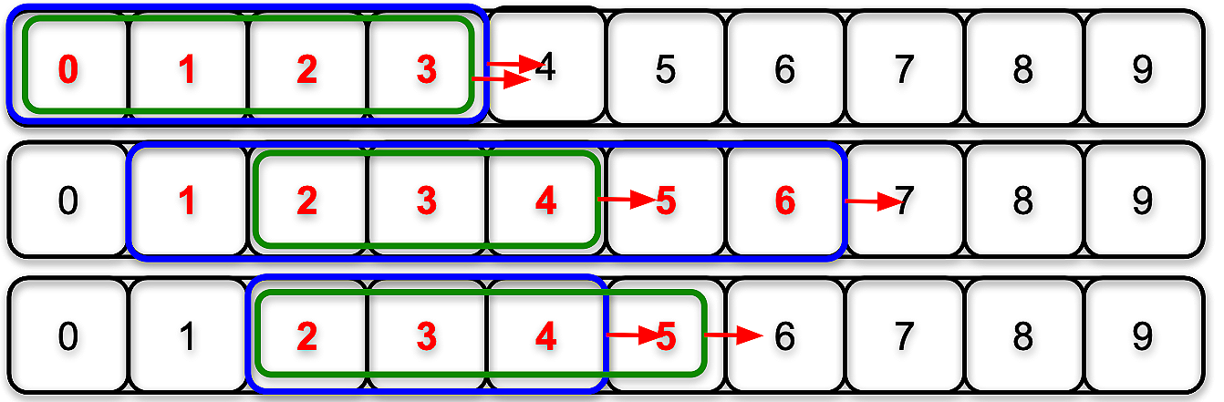
return your_calculation # returns measurement on windowNotice that in the code above we define the range from 0 to the length of the dataset minus the window size plus one. Remember, that the range function is not inclusive, so if the dataset is ten numbers long, and the window size is four, then the range will be [0,10], which only includes the numbers 0-9. Additionally, the total number of windows observed by the program can be defined by the formula len(data)-window_size+1. Therefore, in this example we should expect seven windows to be calculated, as demonstrated below.

Iterating through for i in range(0,len(data)-window_size+1) where len(data) and window_size are 10 and 4.Now that we’ve covered the basic syntax for the sliding window, I’ll show you a specific example for calculating moving averages from minute-by-minute blood glucose data4:
def calculate_moving_average(glucose_data, window_minutes):
    moving_averages = []

    for i in range(0,len(glucose_data) - window_size + 1):
        window = glucose_data[i:i + window_size]
        avg_glucose = np.mean(window)
        moving_averages.append(avg_glucose)

    return moving_averages

min_by_min_glucose = [99, 98, 96, 105, 112, 112, 110, 108, 107, 104]
window_size = 5 # minutes

moving_avg = calculate_moving_average(min_by_min_glucose, window_size)
print("5-min Moving Avgs:", np.round(moving_avg, 1))
Which produces the following output:
5-min Moving Avgs: [102.4 105. 107.4 109.4 109.8 108.2]This basic moving average smooths out short-term fluctuations in blood glucose data, making it easier to identify overall trends. The smoothed data clearly shows blood glucose ramping up over time, which might be obscured by measurement-to-measurement variations in the raw data.
Anomaly Detection With Sliding Windows
A common application of the sliding window technique in wearable data science is anomaly detection. By analyzing patterns in discrete time windows, we can identify when a given individual’s physiological state varies from the norm, whether that's discerning activity from rest, classifying intensity domains during exercise, or detecting the onset of sleep.
The key insight here is that different activities or physiological states have characteristic signatures when viewed over appropriate length time windows. For example, when someone is ill we may expect to see an increased resting heart rate and core body temperature, decrease in HRV, and less movement than the norm for them (due to malaise). In the code block below, I’ll demonstrate how to use sliding windows for anomaly detection, identifying periods of increased heart rate during sleep, which could be a cause for concern.
def detect_health_anomalies(hr_data, timestamps, historical_baseline):
    anomalies = []
    window_size = 60  # 1 hour base window

    for i in range(0,len(hr_data) - window_size + 1):
        hr_window = hr_data[i:i + window_size]
        hr_variability = np.std(hr_window)

        # Calculate window metrics
        window_stats = {
            'mean_hr': np.mean(hr_window),
            'hr_variability': np.std(hr_window),
            'hr_trend': calculate_trend(hr_window),
            'timestamp': timestamps[i + window_size // 2]} # midpoint

        anomaly_score = 0
        # Compare to historical baseline
        # Check for elevated resting heart rate
        if window_stats['mean_hr'] > historical_baseline['mean_hr'] + 2*historical_baseline['hr_std']:
            anomaly_score += 2

        # Check for unusual variability
        if window_stats['hr_variability'] > historical_baseline['variability'] + 2*historical_baseline['var_std']:
            anomaly_score += 1

        # Check for concerning trends
        if abs(window_stats['hr_trend']) > historical_baseline['max_trend']:
            anomaly_score += 1

        # Record significant anomalies
        if anomaly_score >= 2:
            anomaly = {
                'timestamp': window_stats['timestamp'],
                'anomaly_score': anomaly_score,
                'mean_hr': round(window_stats['mean_hr'], 1),
                'expected_hr': round(historical_baseline['mean_hr'], 1),
                'variability': round(window_stats['hr_variability'], 1),
                'concern_level': 'moderate' if anomaly_score < 3 else 'high'}
            anomalies.append(anomaly)

    return anomalies

def calculate_trend(data):
    """Calculate the linear trend in a data series"""
    x = np.arange(len(data))
    slope = np.polyfit(x, data, 1)[0]
    return slope

# Create simulated data showing HR rise during illness
normal_hr = np.random.normal(65, 8, 200)
elevated_hr = np.random.normal(78, 10, 100)
combined_hr = np.concatenate([normal_hr, elevated_hr])
times = pd.date_range('2025-01-01', periods=len(combined_hr), freq='Min')

# Historical baseline (what's normal for this person)
historical_baseline = {
    'mean_hr': 65,
    'hr_std': 5,
    'variability': 8,
    'var_std': 3,
    'max_trend': 0.1}

anomalies = detect_health_anomalies(combined_hr, times, historical_baseline)

print(f"Detected {len(anomalies)} health anomalies:")
for anomaly in anomalies[-2:]: # show last 2
    print(f"Time: {anomaly['timestamp'].strftime('%m/%d %H:%M')}")
    print(f"HR: {anomaly['mean_hr']} BPM (expected: {anomaly['expected_hr']} BPM)")
    print(f"Concern Level: {anomaly['concern_level']}")
    print()
Which produces the following output:
Detected 129 health anomalies:
Time: 01/01 05:29
HR: 76.4 BPM (expected: 65 BPM)
Concern Level: moderate

Time: 01/01 05:30
HR: 76.2 BPM (expected: 65 BPM)
Concern Level: moderate
In the example above, the program detects anomalies in sliding windows by comparing current patterns to historical baselines to identify gradual changes in resting heart rate, unusual heart rate variability patterns, and abnormal heart rate recovery patterns. Notably though, the example above using fixed-size windows, which isn’t always optimal. In the next example we’ll explore variable window sizes.
Variable-Size Sliding Windows
Not all physiological processes occur over fixed time periods. Sleep cycle duration varies night to night, exercise sessions have different durations, and recovery periods during exercise depend on both an individuals fitness level and the exercise intensity. Variable-size sliding windows adapt to these natural variations by expanding and contracting based on the characteristics of the data they iterate over.

Programming a variable-size sliding window is more complicated than a fixed-size window, but it’s worth the extra effort. Instead of forcing all analyses into the same time frame, variable windows adapt to the natural timing of physiological processes, making it a more accurate approach in many real-world scenarios. In the code block below I’ll show you how to implement this approach:
def detect_sleep_periods_variable_window(hr_data, motion_data, timestamps):
    sleep_periods = []
    i = 0
    while i < len(hr_data):
        # Check if current reading suggests sleep onset
        if hr_data[i] < 65 and motion_data[i] < 0.1:  # Low HR and minimal motion
            # Start expanding the window
            sleep_start = i
            sleep_end = i
            # Expand window while sleep criteria are met
            for j in range(i + 1, len(hr_data)):
                if hr_data[j] < 75 and motion_data[j] < 0.2:  # Slightly relaxed criteria
                    sleep_end = j
                else:
                    # Check if this is just a brief interruption
                    if j - sleep_end < 5:  # Less than 5 minutes gap
                        continue
                    else:
                        break
            # Validate sleep period duration
            sleep_duration_minutes = sleep_end - sleep_start
            if sleep_duration_minutes >= 60:  # At least 1 hour
                sleep_period = {
                    'start_time': timestamps[sleep_start],
                    'end_time': timestamps[sleep_end],
                    'duration_hours': round(sleep_duration_minutes / 60, 1),
                    'avg_heart_rate': round(np.mean(hr_data[sleep_start:sleep_end+1]), 1),
                    'sleep_efficiency': calculate_sleep_efficiency(motion_data[sleep_start:sleep_end+1])}
                sleep_periods.append(sleep_period)
            # Move past this sleep period
            i = sleep_end + 1
        else:
            i += 1
    return sleep_periods

def calculate_sleep_efficiency(motion_window):
    low_motion_periods = (np.array(motion_window) < 0.1).sum()
    return round((low_motion_periods / len(motion_window)) * 100, 1)

# Example with simulated overnight data
overnight_times = pd.date_range('2024-01-01 22:00', periods=480, freq='min')  # 8 hours
# Simulate sleep pattern: awake -> light sleep -> deep sleep -> light sleep -> awake
hr_pattern = np.concatenate([np.random.normal(75, 8, 60), np.random.normal(58, 5, 180), np.random.normal(52, 3, 120), np.random.normal(60, 6, 90), np.random.normal(70, 8, 30)])
motion_pattern = np.concatenate([np.random.exponential(0.3, 60), np.random.exponential(0.05, 180), np.random.exponential(0.02, 120), np.random.exponential(0.08, 90), np.random.exponential(0.2, 30)])

sleep_analysis = detect_sleep_periods_variable_window(hr_pattern, motion_pattern, overnight_times)
print("Sleep Period Analysis:")
for period in sleep_analysis:
    print(f"Sleep Duration: {period['duration_hours']} hours")
    print(f"Sleep Time: {period['start_time'].strftime('%H:%M')} - {period['end_time'].strftime('%H:%M')}")
    print(f"Average Sleep HR: {period['avg_heart_rate']} BPM")
    print(f"Sleep Efficiency: {period['sleep_efficiency']}%")
Which produces the following output:
Sleep Period Analysis:
Sleep Duration: 7.0 hours
Sleep Time: 23:00 - 05:59
Average Sleep HR: 57.3 BPM
Sleep Efficiency: 82.6%
The code above detects sleep periods using variable-size sliding windows, which find periods of low heart rate and minimal motion, expand the window as long as sleep criteria are met, and require a minimum duration to avid false positives (ie, make sure sitting idly isn’t mistaken for sleep). Additionally, it calculates sleep efficiency based on motion during the sleep period.
This example builds in complexity from that in the last section, but we’re still just scarping the surface of what you can do with the sliding-window technique.
Advanced Applications of The Sliding Window Technique
As you become more comfortable with sliding window patterns, you can apply them to increasingly sophisticated analyses. For example multi-metric windows can analyze several physiological signals simultaneously, adaptive windows adjust raitheir size based on the data’s characteristics, and overlapping windows can provide more detailed temporal resolution.
In the code block below we’re going to revisit the topic of anomaly detection— where you compare each window to historical patterns to identify unusual physiological events— but with an expanded toolkit that incudes more advanced sliding window techniques:
def advanced_anomaly_detection(hr_data, hrv_data, temp_data, motion_data, timestamps):
    anomalies = []
    base_window_size = 30  # Base window of 30 minutes
    overlap_ratio = 0.5  # 50% overlap between windows
    # Calculate step size for overlapping windows
    step_size = int(base_window_size * (1 - overlap_ratio))
    i = 0
    while i <= len(hr_data) - base_window_size:
        # Adaptive window sizing based on data variability
        window_size = calculate_adaptive_window_size(hr_data[i:i + base_window_size], base_window_size)

        # Ensure we don't exceed data boundaries
        end_idx = min(i + window_size, len(hr_data))

        # Multi-metric window analysis
        window_metrics = analyze_multi_metric_window(
            hr_data[i:end_idx],
            hrv_data[i:end_idx],
            temp_data[i:end_idx],
            motion_data[i:end_idx],
            timestamps[i:end_idx])

        # Detect anomalies using composite scoring
        anomaly_score = calculate_composite_anomaly_score(window_metrics)

        if anomaly_score > 2.5:  # Threshold for significant anomaly
            anomaly = {
                'timestamp': window_metrics['center_time'],
                'window_size_minutes': window_size,
                'anomaly_score': round(anomaly_score, 2),
                'primary_concerns': identify_primary_concerns(window_metrics),
                'metrics': {
                    'hr_mean': round(window_metrics['hr_mean'], 1),
                    'hrv_mean': round(window_metrics['hrv_mean'], 1),
                    'temp_mean': round(window_metrics['temp_mean'], 2),
                    'motion_intensity': round(window_metrics['motion_intensity'], 3)},
                'confidence': calculate_confidence(window_metrics, anomaly_score)}
            anomalies.append(anomaly)

        # Move to next overlapping window
        i += step_size
    return anomalies

def calculate_adaptive_window_size(hr_sample, base_size):
    hr_std = np.std(hr_sample)
    if hr_std < 5:  # Very stable HR
        return max(15, base_size - 10)  # Smaller window
    elif hr_std > 15:  # Highly variable HR
        return min(60, base_size + 20)  # Larger window
    else:
        return base_size  # Standard window

def analyze_multi_metric_window(hr_window, hrv_window, temp_window, motion_window, time_window):
    return {
        # Heart rate metrics
        'hr_mean': np.mean(hr_window),
        'hr_std': np.std(hr_window),
        'hr_trend': np.polyfit(range(len(hr_window)), hr_window, 1)[0],
        'hr_range': np.max(hr_window) - np.min(hr_window),

        # Heart rate variability metrics
        'hrv_mean': np.mean(hrv_window),
        'hrv_std': np.std(hrv_window),
        'hrv_trend': np.polyfit(range(len(hrv_window)), hrv_window, 1)[0],

        # Temperature metrics
        'temp_mean': np.mean(temp_window),
        'temp_std': np.std(temp_window),
        'temp_trend': np.polyfit(range(len(temp_window)), temp_window, 1)[0],

        # Motion metrics
        'motion_intensity': np.mean(motion_window),
        'motion_variability': np.std(motion_window),
        'motion_peaks': len([x for x in motion_window if x > np.mean(motion_window) + 2*np.std(motion_window)]),

        # Temporal information
        'center_time': time_window[len(time_window)//2],
        'window_duration': len(hr_window) }

def calculate_composite_anomaly_score(metrics):
    score = 0

    # Historical baselines (would be personalized in practice)
    baselines = {
        'hr_mean': 65, 'hr_std': 8, 'hrv_mean': 35, 'hrv_std': 12,
        'temp_mean': 98.6, 'temp_std': 0.5, 'motion_intensity': 0.1}

    # Heart rate anomalies
    if abs(metrics['hr_mean'] - baselines['hr_mean']) > 2 * baselines['hr_std']:
        score += 1.5
    if metrics['hr_std'] > baselines['hr_std'] * 1.5:
        score += 1.0
    if abs(metrics['hr_trend']) > 0.5:  # Rapid HR changes
        score += 1.0

    # HRV anomalies (low HRV can indicate stress/illness)
    if metrics['hrv_mean'] < baselines['hrv_mean'] - 2 * baselines['hrv_std']:
        score += 1.5

    # Temperature anomalies
    if abs(metrics['temp_mean'] - baselines['temp_mean']) > 2 * baselines['temp_std']:
        score += 2.0  # Temperature changes are significant

    # Motion pattern anomalies
    if metrics['motion_intensity'] < 0.02 and metrics['hr_mean'] > 70:
        score += 1.0  # High HR with low motion (potential illness)

    # Cross-metric relationships
    if metrics['hr_mean'] > 80 and metrics['hrv_mean'] < 20:
        score += 1.5  # High HR + Low HRV (stress indicator)
    return score

def identify_primary_concerns(metrics):
    concerns = []
    if metrics['temp_mean'] > 99.5:
        concerns.append('elevated_temperature')
    if metrics['hr_mean'] > 85:
        concerns.append('elevated_heart_rate')
    if metrics['hrv_mean'] < 20:
        concerns.append('reduced_hrv')
    if metrics['motion_intensity'] < 0.02 and metrics['hr_mean'] > 70:
        concerns.append('unusual_rest_state')
    if abs(metrics['hr_trend']) > 0.5:
        concerns.append('rapid_hr_changes')
    return concerns if concerns else ['general_anomaly']

def calculate_confidence(metrics, anomaly_score):
    base_confidence = min(anomaly_score / 4.0, 1.0)  # Higher scores = higher confidence
    # Adjust based on data consistency
    if metrics['hr_std'] < 15 and metrics['temp_std'] < 1.0:  # Consistent data
        return min(base_confidence + 0.2, 1.0)
    elif metrics['hr_std'] > 25:  # Very noisy data
        return max(base_confidence - 0.3, 0.1)
    else:
        return base_confidence

# Example usage with simulated data showing illness progression
np.random.seed(42)
time_points = 480
timestamps = pd.date_range('2024-01-01 22:00', periods=time_points, freq='min')
normal_period = 200
illness_period = time_points - normal_period
hr_normal = np.random.normal(65, 8, normal_period)
hr_illness = np.random.normal(75, 12, illness_period) + np.linspace(0, 10, illness_period)
hr_data = np.concatenate([hr_normal, hr_illness])
hrv_normal = np.random.normal(35, 8, normal_period)
hrv_illness = np.random.normal(25, 6, illness_period) - np.linspace(0, 8, illness_period)
hrv_data = np.concatenate([hrv_normal, hrv_illness])
temp_normal = np.random.normal(98.6, 0.3, normal_period)
temp_illness = np.random.normal(99.2, 0.4, illness_period) + np.linspace(0, 1.5, illness_period)
temp_data = np.concatenate([temp_normal, temp_illness])
motion_normal = np.random.exponential(0.15, normal_period)
motion_illness = np.random.exponential(0.05, illness_period)
motion_data = np.concatenate([motion_normal, motion_illness])

# Run advanced anomaly detection
anomalies = advanced_anomaly_detection(hr_data, hrv_data, temp_data, motion_data, timestamps)

print(f"Advanced Anomaly Detection Results:")
print(f"Detected {len(anomalies)} significant physiological anomalies\n")

# Show the most concerning anomalies
for anomaly in sorted(anomalies, key=lambda x: x['anomaly_score'], reverse=True)[:3]:
    print(f"Time: {anomaly['timestamp'].strftime('%m/%d %H:%M')}")
    print(f"Anomaly Score: {anomaly['anomaly_score']} (Confidence: {anomaly['confidence']:.1%})")
    print(f"Window Size: {anomaly['window_size_minutes']} minutes")
    print(f"Primary Concerns: {', '.join(anomaly['primary_concerns'])}")
    print(f"Key Metrics:")
    print(f"  - Heart Rate: {anomaly['metrics']['hr_mean']} BPM")
    print(f"  - HRV: {anomaly['metrics']['hrv_mean']} ms")
    print(f"  - Temperature: {anomaly['metrics']['temp_mean']}°F")
    print(f"  - Motion Level: {anomaly['metrics']['motion_intensity']}")
    print("-" * 50)
Which produces the following output:
Advanced Anomaly Detection Results:
Detected 11 significant physiological anomalies

Time: 01/02 05:15
Anomaly Score: 7.0 (Confidence: 100.0%)
Window Size: 30 minutes
Primary Concerns: elevated_temperature, reduced_hrv, rapid_hr_changes
Key Metrics:
  - Heart Rate: 82.7 BPM
  - HRV: 19.6 ms
  - Temperature: 100.54°F
  - Motion Level: 0.03
--------------------------------------------------
Time: 01/02 05:45
Anomaly Score: 6.0 (Confidence: 100.0%)
Window Size: 30 minutes
Primary Concerns: elevated_temperature, elevated_heart_rate, reduced_hrv
Key Metrics:
  - Heart Rate: 85.0 BPM
  - HRV: 17.2 ms
  - Temperature: 100.74°F
  - Motion Level: 0.048
--------------------------------------------------
Time: 01/02 04:00
Anomaly Score: 4.5 (Confidence: 100.0%)
Window Size: 30 minutes
Primary Concerns: elevated_temperature, rapid_hr_changes
Key Metrics:
  - Heart Rate: 82.5 BPM
  - HRV: 20.9 ms
  - Temperature: 100.08°F
  - Motion Level: 0.053
The code block above implements an advanced anomaly detection system using multi-metric, overlapping, and adaptive windows that adjust size based on heart rate variability (more variability leads to larger windows for more stable analyses). During each window the program analyzes multiple physiological metrics, calculates anomaly scores based on various physiological indicators, and identifies areas of concert with confidence scores based on data quality and consistency.
Two-Pointer Techniques — Spotting Connections In Time-Series Data
The two-pointer pattern is a useful technique for finding relationships between data points, especially when you need to analyze pairs of measurements or identify patterns that span across different time periods. Unlike sliding windows that analyze consecutive data points, two-pointer algorithms can examine data points that are distance from one another, making them perfect for analyzing relationships between non-adjacent measurements.
In wearable data science, two-pointer techniques excel at problems like identifying sleep and wake patterns, analyzing heart rate (or muscle oxygenation and VO2) response and recovery relationships, or detecting correlated changes between different physiological metrics. The key advantage is efficiency—instead of checking every possible pair of data points (which would be computationally expensive), two-pointer techniques use intelligent movement strategies to find meaningful relationships quickly.
The fundamental concept involves maintaining two "pointers" (indices) that move through your data according to specific rules. These pointers might start at opposite ends of your dataset and move toward each other, or they might both start at the beginning and move at different speeds. The movement strategy depends on what relationships you're trying to find.
The basic programming syntax to implement the two-pointer technique, in all of these cases, is as follows:
def two_pointer_analysis(data, target_condition):
    left = 0
    right = len(data) - 1
    results = []

    while left < right:
        # Analyze current pair
        if meets_condition(data[left], data[right], target_condition):
            results.append((left, right, data[left], data[right]))
            left += 1
            right -= 1
        elif needs_left_adjustment(data[left], data[right], target_condition):
            left += 1
        else:
            right -= 1
    return results
Now, let’s apply this concept to heart rate recovery analysis, where the goal is to find pairs of heart rate peaks and corresponding recovery periods using the two-pointer technique.
def find_optimal_workout_recovery_pairs(hr_data, timestamps, recovery_target=20):
    workout_recovery_pairs = []

    # Find potential workout peaks (high heart rate periods)
    potential_peaks = []
    for i, hr in enumerate(hr_data):
        if hr > 100:  # Potential exercise heart rate
            potential_peaks.append((i, hr))

    # Use two pointers to find recovery relationships
    for peak_idx, peak_hr in potential_peaks:
        # Look for recovery within next 30 minutes
        search_end = min(peak_idx + 30, len(hr_data))

        for recovery_idx in range(peak_idx + 5, search_end):  # At least 5 min later
            recovery_hr = hr_data[recovery_idx]
            hr_drop = peak_hr - recovery_hr

            if hr_drop >= recovery_target:
                recovery_time = recovery_idx - peak_idx
                pair = {
                    'peak_time': timestamps[peak_idx],
                    'peak_hr': peak_hr,
                    'recovery_time': timestamps[recovery_idx],
                    'recovery_hr': recovery_hr,
                    'hr_drop': hr_drop,
                    'recovery_duration_min': recovery_time}
                workout_recovery_pairs.append(pair)
                break  # Found recovery for this peak
    return workout_recovery_pairs

# Example with simulated workout data
workout_times = pd.date_range('2024-01-01 08:00', periods=90, freq='min')
hr_workout = np.concatenate([np.random.normal(75, 5, 10),  np.random.normal(140, 8, 15), np.random.normal(85, 5, 10), np.random.normal(150, 10, 15), np.random.normal(90, 8, 10),])

recovery_analysis = find_optimal_workout_recovery_pairs(hr_workout, workout_times)
print("Workout Recovery Analysis:")
for pair in recovery_analysis:
    print(f"Peak: {pair['peak_hr']} BPM at {pair['peak_time'].strftime('%H:%M')}")
    print(f"Recovery: {pair['recovery_hr']} BPM at {pair['recovery_time'].strftime('%H:%M')}")
    print(f"HR Drop: {pair['hr_drop']} BPM in {pair['recovery_duration_min']} minutes\n")
Which produces the following (truncated) output:
Peak: 152.13293707372938 BPM at 08:35
Recovery: 129.96137635593246 BPM at 08:47
HR Drop: 22.171560717796922 BPM in 12 minutes

Peak: 150.01205475362224 BPM at 08:36
Recovery: 129.96137635593246 BPM at 08:47
HR Drop: 20.05067839768978 BPM in 11 minutes
The analysis above can reveal some interesting insights. Faster heart rate recovery generally indicates better cardiovascular fitness, while slower recovery might suggest overtraining, fatigue, or declining fitness levels. By automatically identifying these patterns, you can track chances in fitness over time.
Spotting Sleep-Wake Transitions With the Two-Pointer Technique
Two-pointer techniques are particularly effective for analyzing complementary physiological states like sleep and wake periods. By examining the relationships between bedtime and wake-up patterns, you can identify optimal sleep durations, detect sleep debt patterns, and analyze how sleep timing affects next-day performance.
In the code block below, we’ll implement a program that uses a more advanced version of the two-pointer technique to find relationships between sleep onset and wake-up times, sleep duration and next day performance, and bedtime consistency and sleep quality.
def analyze_sleep_wake_patterns(activity_data, hr_data, timestamps):
    sleep_events = []
    wake_events = []

    # Identify sleep and wake events
    for i, (activity, hr) in enumerate(zip(activity_data, hr_data)):
        if activity == 'sleep' and hr < 65:
            if i == 0 or activity_data[i-1] != 'sleep':  # Sleep onset
                sleep_events.append((i, timestamps[i], hr))
        elif activity != 'sleep' and hr > 70:
            if i > 0 and activity_data[i-1] == 'sleep':  # Wake up
                wake_events.append((i, timestamps[i], hr))

    # Use two pointers to match sleep-wake pairs
    sleep_wake_pairs = []
    sleep_ptr = 0
    wake_ptr = 0
    while sleep_ptr < len(sleep_events) and wake_ptr < len(wake_events):
        sleep_idx, sleep_time, sleep_hr = sleep_events[sleep_ptr]
        wake_idx, wake_time, wake_hr = wake_events[wake_ptr]

        # Check if this wake event follows this sleep event
        if wake_time > sleep_time and (wake_time - sleep_time).total_seconds() < 12 * 3600:  # Within 12 hours
            sleep_duration = (wake_time - sleep_time).total_seconds() / 3600  # Hours

            # Calculate sleep quality metrics
            sleep_period_hr = hr_data[sleep_idx:wake_idx]
            avg_sleep_hr = np.mean(sleep_period_hr)
            hr_stability = np.std(sleep_period_hr)

            pair = {
                'sleep_time': sleep_time,
                'wake_time': wake_time,
                'duration_hours': round(sleep_duration, 1),
                'avg_sleep_hr': round(avg_sleep_hr, 1),
                'sleep_stability': round(hr_stability, 1),
                'sleep_efficiency': calculate_sleep_efficiency_score(sleep_duration, hr_stability)}
            sleep_wake_pairs.append(pair)
            sleep_ptr += 1
            wake_ptr += 1
        elif wake_time < sleep_time:
            wake_ptr += 1
        else:
            sleep_ptr += 1
    return sleep_wake_pairs

def calculate_sleep_efficiency_score(duration, stability):
    """Calculate sleep efficiency based on duration and heart rate stability"""
    duration_score = min(duration / 8, 1) * 50  # Optimal 8 hours
    stability_score = max(0, (20 - stability) / 20) * 50  # Lower variability is better
    return round(duration_score + stability_score, 1)

# Simulate 3 days of sleep-wake data
daily_times = pd.date_range('2024-01-01 00:00', periods=72, freq='h')  # 3 days
activity_pattern = (['sleep'] * 8 + ['awake'] * 16) * 3  # 8 hours sleep, 16 awake
hr_pattern = []

for activity in activity_pattern:
    if activity == 'sleep':
        hr_pattern.append(np.random.normal(58, 6))
    else:
        hr_pattern.append(np.random.normal(75, 12))

sleep_analysis = analyze_sleep_wake_patterns(activity_pattern, hr_pattern, daily_times)
print("Sleep-Wake Pattern Analysis:")
for i, night in enumerate(sleep_analysis, 1):
    print(f"Night {i}:")
    print(f"  Sleep: {night['sleep_time'].strftime('%m/%d %H:%M')} - {night['wake_time'].strftime('%m/%d %H:%M')}")
    print(f"  Duration: {night['duration_hours']} hours")
    print(f"  Sleep HR: {night['avg_sleep_hr']} BPM (stability: {night['sleep_stability']})")
    print(f"  Efficiency Score: {night['sleep_efficiency']}/100\n")
Which produces the following output:
Sleep-Wake Pattern Analysis:
Night 1:
  Sleep: 01/01 00:00 - 01/01 08:00
  Duration: 8.0 hours
  Sleep HR: 56.4 BPM (stability: 5.8)
  Efficiency Score: 85.6/100

Night 2:
  Sleep: 01/02 00:00 - 01/02 08:00
  Duration: 8.0 hours
  Sleep HR: 56.4 BPM (stability: 5.2)
  Efficiency Score: 87.0/100

Night 3:
  Sleep: 01/03 00:00 - 01/03 08:00
  Duration: 8.0 hours
  Sleep HR: 51.7 BPM (stability: 3.1)
  Efficiency Score: 92.3/100
In addition to spotting relationships in sleep data, like the example above, more advanced versions of the two-pointer technique can be used to find correlations between different physiological metrics over varying time scales, which can lead to interesting insights like how yesterday’s sleep quality affects today's HRV, or how morning exercise intensity correlates with evening recovery metrics.
Closing Thoughts
The sliding window and two-pointer techniques represent foundational algorithmic patterns used in wearable data. What makes these approaches so useful is their adaptability. The same sliding window pattern that calculates a simple moving average can be extended to detect sleep onset, identify exercise recovery periods, or flag concerning health anomalies. Similarly, two-pointer techniques that find basic correlations between metrics can evolve into sophisticated systems for predicting performance, optimizing recovery, or providing early health warnings.
Once you understand the underlying logic behind these two algorithms, adapting them to new challenges becomes intuitive. The key is to start simple, understand the fundamentals, then gradually build complexity as your specific use cases demand.
If you enjoyed this article and want to see more like it, let me know in the comments below. Additionally, if you want to see some examples of how i’m implementing these algorithms, and others, in my own work check out AssessWorks, a web-based platform democratizing advanced physiological analyses.
Interested in working together? I advise small companies, startups, and VC firms on topics ranging from biosensor development, multiomics and biometric data analysis, network modeling, and product strategy. Contact eva♦peiko♦@gmail.com (replace the ♦ with n) for consulting inquiries or newsletter sponsorship opportunities.
All of these guides are freely available in my Bioinformatics Toolkit— a growing collection of bioinformatics tutorials, project guides, analytics tools, and article’s I’ve created to help make bioinformatics more approachable and accessible.
PhysioNexus is a open source tool that transforms complex time series data into intuitive network visualizations showing cause-and-effect relationships between physiological data, environmental variables, and external load measurements.If you’re interested in learning more you can check out the following non-technical guide: Breaking Biometric Babel.
Unlike general-purpose programming algorithms that focus on abstract data structures, algorithms geared specially for wearable data need to content with the unique characteristics of physiological signals — temporal dependences (ie, what happened in previous measurements affects current interpretation), noise and artifacts from sensor-specific limitations, a lack of stationary in data, and often the need to make real-time decisions from streaming data (as opposed to analyzing data retroactively).
All of the code blocks used in this tutorial assume you’re already imported pandas and numpy as pd and np respectively.