


Introduction To Time Series Analysis & Forecasting
Understanding Time Series Data To Make Better Predictions About The Future


🧬 Introduction To Time Series Analysis & Forecasting
Time series analysis and time series forecasting are interesting but often neglected topics in applied machine learning. Time series analysis and forecasting are often neglected because time series data can be cumbersome to work with, and many popular uses of machine learning do not explicitly consider time as an underlying data structure.
However, if you’re interested in biomedical and human performance applications of machine learning, time series analysis and forecasting are immensely important because many biological datasets involve a time component. For example, if you wanted to analyze your health data from an Apple Watch or make predictions based on that data, you would rely on time series analysis and forecasting methodologies respectively.
Despite many machine learning models not explicitly considering time as an underlying data structure, time still plays a role. For example, predictions about future events are often made despite outcomes not being known until a future date. This differs from time series analysis and forecasting because all past observations in the dataset are treated equally. Time series data, on the other hand, has an explicit order, and time provides an additional constraint and underlying structure to the data. For example, in the image below we have two small datasets. The dataset on the left contains a collection of observations without a time component. The dataset on the right, on the other hand, is a collection of observations taken sequentially in time.

Before moving on, I will cover some fundamental terms for time series data. Anytime we work with time series data, the current time is defined as t. Thus, previous events are negative relative to our current time and are denoted as t-. For example, at time t, the most recent observation would be t-1, and the observation before that is t-2. Previous observations are often referred to as lags, so a lag of 5 (lag=5) would be synonymous with t-5. On the other hand, future events relative to the current time are denoted with t+, such that the next observation relative to t is t+1, and so on.
🧬 Time Series Analysis Vs. Forecasting
Time series analysis and forecasting are often used interchangeably despite not being synonymous. Simply put, time series analysis is the process of dissecting and understanding time series data. In contrast, time series forecasting is the process of using time series data to predict future events. Keep in mind these processes are linked in that time series analysis can improve your ability to make future predictions via time series forecasting.
The core purpose of time series analysis is to develop qualitative or qualitative models that provide plausible descriptions from sample data. In other words, time series analysis answers the questions such as "what?", "why?", and "how?". An example of time series analysis would be looking at a patient's EKG trend to determine if they previously experienced atrial fibrillation or analyzing an athlete's VO2 and NIRS data after a workout to identify their physiologic limitation.

On the other hand, time series forecasting involves taking models based on historical data (like the time series trends above) and using them to make predictions about the future. An example of time series forecasting would be predicting if a patient is likely to experience atrial fibrillation based on their historic EKG data or predicting an athlete's proximity to task failure during a race based on the data already recorded up to that point in the event.
An important distinction between time series analysis and time series forecasting is that with time series forecasting you make predictions about an unknown and unknowable future based solely on the events that have already occurred. To the extent that the future resembles the past, you can make accurate predictions. Still, this method has its limitations when exploring new terrain, as is often the case when analyzing complex biological data that was not previously available.
🧬 Dissecting Time Series Data
Time series data follow somewhat formulaic patterns, which you can identify to better understand what is happening in your dataset. Three common patterns you should aim to spot are your data's level, trend, and seasonality. Below I’ll demonstrate these three patterns using datasets recorded with a NNOXX One wearable device.
“The main features of many time series are trends and seasonal variations… Another important feature of most time series is that observations close together in time tend to be correlated.” -Metcalfe & Cowpertwait, 2009
The level (i.e., baseline) in a time series dataset is a theoretical straight line that would span the x-axis if the baseline value for the series continued in a straight line. For example, in the image below, you’ll find a time series dataset with my muscle oxygenation (SmO2) level during a short workout. My resting SmO2 level is ~65% when I start recording my data. Thus, this is my level (baseline), highlighted in red in the image below.

The trend in a time series dataset refers to the data's acute increasing or decreasing behavior over time. For example, in the image below, you can see my muscle oxygenation (SmO2) level during a short sprint. During the sprint, my SmO2 declines, as highlighted in red, and during the recovery period, my SmO2 increases, as highlighted in pink.

Seasonality in a time series dataset refers to cycles and patterns in the data that repeat themselves over time. For example, in the image below, you can see a repeating cycle of deoxygenation (red) and reoxygenation (pink) in my SmO2 data as I perform an interval training workout.

All time series datasets have a baseline level, but not all have trends or seasonality. Additionally, some time series datasets contain noise, which are variations in the data that the model cannot explain. Time series decomposition is the process of dissecting a time series into its constituent components to better understand it and improve analysis and forecasting abilities. In future newsletter, I’ll cover the decomposition of time series data into a level, trend(s), and seasonality.
🧬 Modeling Time Series Data
You can frame time series analysis and forecasting as a supervised machine learning problem, where you have input variables (x) and output variables (y), and you use an algorithm to learn the mapping function that transforms an input variable to its corresponding output variable. The generic formula for a mapping function is as follows: y = f(x)
Once you understand the mapping function, f(x), you can use it to make predictions about new, previously unseen data. However, before doing so, you need to re-format your time series data so that you can perform supervised machine learning to learn the mapping function mentioned above. One way to do this is with the sliding window method, also known as the lag method, which uses the previous time-step in a dataset to predict the next time-step. Below you’ll find a demonstration using the sliding window method to re-organize a simple univariate time series dataset:

After using the sliding window method to re-organize our time series data, we can use the re-organized data to train a supervised machine learning model. However, it’s worth noting that the order of observations must be persevered to train the model. Additionally, best practices dictate that we delete the last row in the re-organized dataset since we do not have a corresponding output value to pair it with.
We can also use the sliding window method for multi-step forecasting, where two or more future time steps are predicted, as demonstrated in the example below:

In the example above, I used the sliding window method to re-organize a univariate time series dataset, which only had a single observed variable (in this case, SmO2) at each time step. However, we can also use the sliding window method to re-organize multivariate data, with two variables at each time step.
“Multivariate time series analysis considers simultaneously multiple time series… It is, in general, much more complicated than univariate time series analysis.” -Tsay, 2013
Below you’ll find a demonstration using the sliding window method to re-organize a multivariate time series dataset:
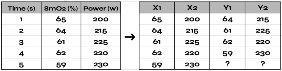
Notice, in the example above, we are predicting two output measurements at the next time step. Few machine learning methods can handle predicting multiple output variables from a time series dataset (artificial neural networks being an exception). As a result, it’s more common to re-organize our time series data to only predict just one output measurement, which you’ll see in the example below:

In the examples above, I showed you how to re-organize time series data before performing supervised machine learning. I prefer to re-organize my data in Google Sheets or Excel manually. However, if you're working with large datasets or performing time series analysis and forecasting frequently, it's worth learning to automate these tasks, which I'll cover in a future newsletter.
👉 If you have any questions about the content in this newsletter please let me know in the comment section below.
👉 If you liked this post, don’t forget to leave a like ❤️. It helps more people discover this newsletter on Substack. The button is located towards the bottom of this email.
👉 If you enjoy reading this newsletter, please share it with friends!