Evaluation Metrics for Biological Classification Problems

🧬 Introduction to Performance Metrics in Biomedical Machine Learning

In biomedical research and clinical diagnostics, machine learning algorithms are increasingly being used to classify biological states, predict disease outcomes, and identify molecular signatures. The accuracy of these predictions can have profound implications for patient care, making the proper evaluation of model performance crucial. While my previous discussion on resampling methods covered how to estimate a model's performance on unseen data, this article delves into the statistical techniques used to quantify that performance.

The distinction between evaluation methods and metrics is particularly important in biological contexts. Evaluation methods like cross-validation tell us how well our model might generalize to new patients or samples, while evaluation metrics tell us specifically what kinds of errors we're making – critical information when those errors could mean missed diagnoses or unnecessary treatments.

🧬 Understanding Classification in Biological Systems

Before diving into specific metrics, let's consider what classification means in biological systems. Take, for example, the classification of diabetes patients. The biological reality is far more complex than a simple binary outcome – patients exist on a spectrum of insulin sensitivity and glucose regulation. However, for clinical decision-making, we often need to make binary classifications: does this patient require intervention or not?

This complexity makes the choice of evaluation metrics particularly important. A false negative in cancer detection has different implications than a false positive in an antibiotic resistance test. Let's explore these metrics using synthetic patient data that mirrors real-world biological complexity.

🧬 Classification Accuracy: A Basic but Limited Metric

Classification accuracy represents the percentage of correct predictions across all cases. While straightforward, its limitations become apparent in biological contexts where class imbalances are common. Consider a rare genetic disorder affecting 1 in 1000 people. A model that simply predicts "no disorder" for everyone would achieve 99.9% accuracy while being clinically useless.

Below you'll find sample code using classification accuracy (in conjunction with k-fold cross-validation) to determine the effectiveness of a machine learning model:

# Import libraries 
import numpy as np
import pandas as pd
from sklearn.model_selection import KFold
from sklearn.model_selection import cross_val_score
from sklearn.linear_model import LogisticRegression

# Generate synthetic patient data
np.random.seed(42)
n_patients = 1000

# Create features that mirror real biological parameters
data = pd.DataFrame({
    'glucose_fasting': np.random.normal(100, 20, n_patients), # mg/dL
    'hba1c': np.random.normal(5.7, 0.5, n_patients),          # %
    'bmi': np.random.normal(25, 4, n_patients),               # kg/m²
    'age': np.random.normal(50, 15, n_patients)})             # years


# Generate diabetes status based on biological relationships
probability = 1 / (1 + np.exp(-(
    -15 +                               # baseline
    0.05 * data['glucose_fasting'] +    # glucose effect
    1.5 * data['hba1c'] +               # HbA1c effect
    0.1 * data['bmi'] +                 # BMI effect
    0.02 * data['age'])))               # age effect

data['diabetes'] = (np.random.random(n_patients) < probability).astype(int)

# Prepare data for modeling
x,y = data.drop('diabetes', axis=1), data['diabetes']

# Evaluate using k-fold cross-validation
kfold = KFold(n_splits=10, shuffle=True, random_state=42)
model = LogisticRegression(solver='liblinear')
results = cross_val_score(model, x, y, cv=kfold, scoring='accuracy')
print(f'Mean Accuracy: {results.mean()*100:.1f}%')
print(f'Standard Deviation: {results.std()*100:.1f}%')

Which produces the following outputs:

• Mean Accuracy: 83.7%

• Standard Deviation: 4.3%

🧬 The Confusion Matrix: Understanding Error Types

In biological classification, the type of error often matters more than the overall error rate. A confusion matrix breaks down predictions into four categories that have distinct biological and clinical implications:

• True Positives (TP): Correctly identified cases (e.g., diagnosed diabetics)

• False Positives (FP): Type I errors (e.g., healthy patients misdiagnosed as diabetic)

• False Negatives (FN): Type II errors (e.g., missed diabetes cases)

• True Negatives (TN): Correctly identified controls

This breakdown is particularly valuable in biomedical contexts where the cost of different types of errors varies dramatically. For instance, in cancer screening, false negatives (missed cancers) are generally considered more serious than false positives (unnecessary follow-up tests).

Let's generate a confusion matrix using our synthetic patient data:

# Import libraries
from sklearn.metrics import confusion_matrix
import seaborn as sns
import matplotlib.pyplot as plt
from sklearn.model_selection import train_test_split

# Split data and fit model
X_train, X_test, y_train, y_test = train_test_split(X, y, test_size=0.3, random_state=42)
model = LogisticRegression(solver='liblinear')
model.fit(X_train, y_train)

# Generate and visualize confusion matrix
predictions = model.predict(X_test)
cm = confusion_matrix(y_test, predictions)

plt.figure(figsize=(8, 6))
sns.heatmap(cm, annot=True, fmt='d', cmap='Blues')
plt.title('Confusion Matrix for Diabetes Classification')
plt.ylabel('True Label')
plt.xlabel('Predicted Label')

Which produces the following output:

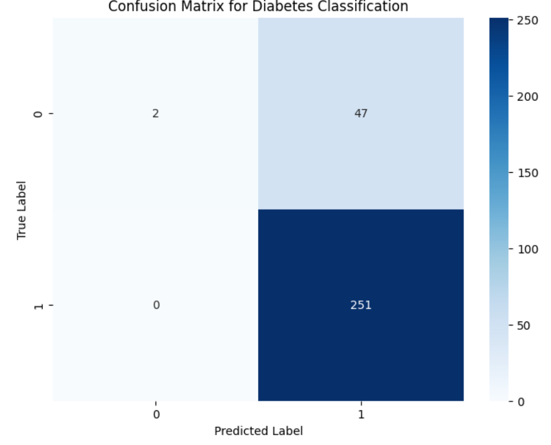
The top left corner of the image above are the true positive, the bottom left are the false positives, the top right are the false negatives, and the bottom are the true negatives. After generating a confusion matrix, you can also manually calculate the precision, recall, and f1-score, as demonstrated In the next section.

🧬 Precision, Recall, and the F1-Score: Balancing Different Types of Errors

In biological classification, we often need to balance competing objectives. Precision (positive predictive value) measures how many of our positive predictions are correct, while recall (sensitivity) measures how many actual positive cases we identified. These metrics have direct biological interpretations. For example, take precision and recall, defined by the formulas below:

Precision = TP / (TP + FP)

Recall = TP / (TP + FN)

In diagnostic terms, precision tells us of the patients we diagnosed with the condition, what proportion actually had it?" Recall, on the other hand, tells us of all of the patients who had the condition, what proportion did we correctly identify?"

The F1-score provides a single metric combining precision and recall, useful for comparing different models or choosing optimal classification thresholds. This is particularly relevant when working with biological data where both false positives and false negatives have significant consequences.

from sklearn.metrics import classification_report
# Generate classification report
print(classification_report(y_test, predictions))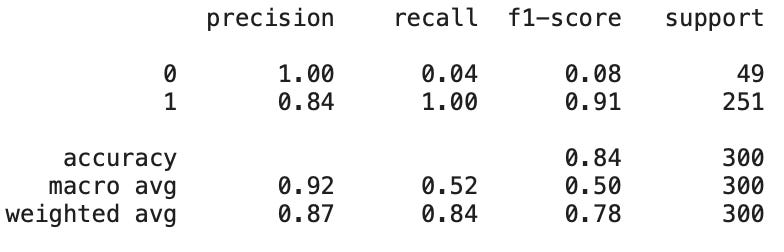

🧬 ROC Curves and AUC: Evaluating Diagnostic Power

The Receiver Operating Characteristic (ROC) curve has its origins in signal detection theory and is particularly well-suited for evaluating diagnostic tests. The Area Under the ROC Curve (AUC) measures a model's ability to discriminate between classes across all possible classification thresholds.

In biological terms, the ROC curve plots the tradeoff between sensitivity (true positive rate) and specificity (true negative rate) as we vary the classification threshold. This is especially relevant for diagnostic tests where we might want to adjust the threshold based on the clinical context – for example, using a more sensitive threshold for initial screening versus a more specific threshold for definitive diagnosis.

from sklearn.metrics import roc_curve, auc
import matplotlib.pyplot as plt

# Generate probability predictions
y_prob = model.predict_proba(X_test)[:, 1]

# Calculate ROC curve
fpr, tpr, thresholds = roc_curve(y_test, y_prob)
roc_auc = auc(fpr, tpr)

# Plot ROC curve
plt.figure(figsize=(8, 6))
plt.plot(fpr, tpr, color='darkorange', lw=2, 
         label=f'ROC curve (AUC = {roc_auc:.2f})')
plt.plot([0, 1], [0, 1], color='navy', lw=2, linestyle='--')
plt.xlim([0.0, 1.0])
plt.ylim([0.0, 1.05])
plt.xlabel('False Positive Rate')
plt.ylabel('True Positive Rate')
plt.title('ROC Curve for Diabetes Classification')
plt.legend(loc="lower right")

Which produces the following output:

🧬 Logistic Loss: Measuring Prediction Confidence

Logistic loss (log loss) is particularly relevant in biological classification because it considers not just the correctness of predictions but also their confidence. This is crucial in medical diagnostics where we often need to know not just whether a patient is classified as diseased or healthy, but how confident we are in that classification.

For instance, in genetic testing, we might want to distinguish between clear positive results and borderline cases that require additional testing. Log loss penalizes models that are very confident about incorrect predictions, making it especially useful for evaluating diagnostic algorithms where calibrated probability estimates are important.

from sklearn.metrics import log_loss

# Calculate log loss
log_loss_value = log_loss(y_test, y_prob)
print(f'Log Loss: {log_loss_value:.3f}')

Which produces the following output:

• Log Loss: 0.401

🧬 Conclusion: Choosing Appropriate Metrics for Biological Classification

The choice of evaluation metrics should be guided by the biological context and clinical implications of classification errors. While accuracy provides a simple overview, more nuanced metrics like precision, recall, and AUC offer insights that are directly relevant to biological decision-making.

For diagnostic applications, consider using:

• ROC AUC for overall diagnostic power

• Precision and recall when the costs of false positives and negatives are different

• Log loss when probability calibration is important

Remember that biological systems are inherently complex and variable. A combination of metrics, interpreted in the context of biological knowledge and clinical requirements, will provide the most complete evaluation of classification performance.